Reinforcement Learning: Learn How Agents Optimize Rewards
•
3 j'aime•854 vues

( Machine Learning & Deep Learning Specialization Training: https://goo.gl/5u2RiS ) This CloudxLab Reinforcement Learning tutorial helps you to understand Reinforcement Learning in detail. Below are the topics covered in this tutorial: 1) What is Reinforcement? 2) Reinforcement Learning an Introduction 3) Reinforcement Learning Example 4) Learning to Optimize Rewards 5) Policy Search - Brute Force Approach, Genetic Algorithms and Optimization Techniques 6) OpenAI Gym 7) The Credit Assignment Problem 8) Inverse Reinforcement Learning 9) Playing Atari with Deep Reinforcement Learning 10) Policy Gradients 11) Markov Decision Processes

Recommandé
Contenu connexe
Tendances
Tendances (20)
Similaire à Reinforcement Learning: Learn How Agents Optimize Rewards
Similaire à Reinforcement Learning: Learn How Agents Optimize Rewards (20)
Plus de CloudxLab
Plus de CloudxLab (20)
Dernier
Dernier (20)
Reinforcement Learning: Learn How Agents Optimize Rewards
- 2. Reinforcement Learning ● Reinforcement Learning has been around since 1950s and ○ Produced many interesting applications over the years ○ Like TD-Gammon, a Backgammon playing program Reinforcement Learning
- 3. Reinforcement Learning ● In 2013, researchers from an English startup DeepMind ○ Demonstrated a system that could learn to play ○ Just about any Atari game from scratch and ○ Which outperformed human ○ It used only row pixels as inputs and ○ Without any prior knowledge of the rules of the game ● In March 2016, their system AlphaGo defeated ○ Lee Sedol, the world champion of the game of Go ○ This was possible because of Reinforcement Learning Reinforcement Learning
- 4. Reinforcement Learning ● In this chapter, we will learn about ○ What Reinforcement Learning is and ○ What it is good at Reinforcement Learning
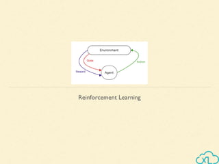
- 5. Reinforcement Learning Learning to Optimize Rewards Reinforcement Learning
- 6. Reinforcement Learning ● In Reinforcement Learning ○ A software agent makes observations and ○ Takes actions within an environment and ○ In return it receives rewards Learning to Optimize Rewards
- 7. Reinforcement Learning Goal? Learning to Optimize Rewards
- 8. Reinforcement Learning Goal Learn how to take actions in order to maximize reward Learning to Optimize Rewards
- 9. Reinforcement Learning ● In short, the agent acts in the environment and ○ Learns by trial and error to ○ Maximize its reward Learning to Optimize Rewards
- 10. Reinforcement Learning So how can we apply this in real-life applications? Learning to Optimize Rewards
- 11. Reinforcement Learning Learning to Optimize Rewards - Walking Robot
- 12. Reinforcement Learning ● Agent - Program controlling a walking robot ● Environment - Real world ● The agent observes the environment through a set of sensors such as ○ Cameras and touch sensors ● Actions - Sending signals to activate motors Learning to Optimize Rewards - Walking Robot
- 13. Reinforcement Learning ● It may be programmed to get ○ Positive rewards whenever it approaches the target destination and ○ Negative rewards whenever it ■ Wastes time ■ Goes in the wrong direction or ■ Falls down Learning to Optimize Rewards - Walking Robot
- 14. Reinforcement Learning Learning to Optimize Rewards - Ms. Pac-Man
- 15. Reinforcement Learning ● Agent - Program controlling Ms. Pac-Man ● Environment - Simulation of the Atari game ● Actions - Nine possible joystick positions ● Observations - Screenshots ● Rewards - Game points Learning to Optimize Rewards - Ms. Pac-Man
- 16. Reinforcement Learning Learning to Optimize Rewards - Thermostat
- 17. Reinforcement Learning ● Agent - Thermostat ○ Please note, the agent does not have to control a ○ Physically (or virtually) moving thing ● Rewards - ○ Positive rewards whenever agent is close to the target temperature ○ Negative rewards when humans need to tweak the temperature ● Important - Agent must learn to anticipate human needs Learning to Optimize Rewards - Thermostat
- 18. Reinforcement Learning Learning to Optimize Rewards - Auto Trader
- 19. Reinforcement Learning ● Agent - ○ Observes stock market prices and ○ Decide how much to buy or sell every second ● Rewards - The monetary gains and losses Learning to Optimize Rewards - Auto Trader
- 20. Reinforcement Learning ● There are many other examples such as ○ Self-driving cars ○ Placing ads on a web page or ○ Controlling where an image classification system ■ Should focus its attention Learning to Optimize Rewards
- 21. Reinforcement Learning ● Note that there may not be any positive rewards at all ● For example ○ The agent may move around in a maze ○ Getting a negative reward at every time step ○ So it better find the exit as quickly as possible Learning to Optimize Rewards
- 23. Reinforcement Learning ● The algorithm used by the software agent to ○ Determine its actions is called its policy ● For example, the policy could be a neural network ○ Taking observations as inputs and ○ Outputting the action to take Policy Search
- 24. Reinforcement Learning ● The policy can be any algorithm we can think of ○ And it does not even have to be deterministic ● For example, consider a robotic vacuum cleaner ○ Its reward is the amount of dust it picks up in 30 minutes ● Its policy could be to ○ Move forward with some probability p every second or ○ Randomly rotate left or right with probability 1 – p ○ The rotation angle would be a random angle between –r and +r ● Since this policy involves some randomness ○ It is called a stochastic policy Policy Search
- 25. Reinforcement Learning ● The robot will have an erratic trajectory, which guarantees that ○ It can get to any place it can reach and ○ Pick up all the dust ● The question is: how much dust will it pick up in 30 minutes? Policy Search
- 26. Reinforcement Learning How would we train such a robot? Policy Search
- 27. Reinforcement Learning ● There are just two policy parameters which we can tweak ○ The probability p and ○ The angle range r Policy Search
- 28. Reinforcement Learning ● One possible learning algorithm could be to ○ Try out many different values for these parameters, and ○ Pick the combination that performs best ● This is the example of policy search using a brute force approach Policy Search - Brute Force Approach Four points in policy space and the agent’s corresponding behavior
- 29. Reinforcement Learning ● When the policy space is too large then ○ Finding a good set of parameters this way is like ○ Searching for a needle in a gigantic haystack Policy Search - Brute Force Approach Four points in policy space and the agent’s corresponding behavior
- 30. Reinforcement Learning ● Another way to explore the policy space is to ○ Use genetic algorithms ● For example ○ Randomly create a first generation of 100 policies and ○ Try them out, then “kill” the 80 worst policies and ○ Make the 20 survivors produce 4 offspring each ● An offspring is just a copy of its parent ○ Plus some random variation Policy Search - Genetic Algorithms
- 31. Reinforcement Learning ● The surviving policies plus their offspring together ○ Constitute the second generation ● Continue to iterate through generations this way ○ Until a good policy is found Policy Search - Genetic Algorithms
- 32. Reinforcement Learning ● Another approach is to use ○ Optimization Techniques ● Evaluate the gradients of the rewards ○ With regards to the policy parameters ○ Then tweaking these parameters by following the ○ Gradient toward higher rewards (gradient ascent) ● This approach is called policy gradients Policy Search - Optimization Techniques
- 33. Reinforcement Learning ● Let’s understand this with an example ● Going back to the vacuum cleaner robot example, we can ○ Slightly increase p and evaluate ○ Whether this increases the amount of dust ○ Picked up by the robot in 30 minutes ○ If it does, then increase p some more, or ○ Else reduce p Policy Search - Optimization Techniques
- 34. Reinforcement Learning Introduction to OpenAI Gym
- 35. Reinforcement Learning ● To train an agent in Reinforcement Learning ○ We need a working environment ● For example, if we want agent to run how to play Atari game, ○ We will need a Atari game simulator ● OpenAI gym is a toolkit that provides wide variety of simulations like ○ Atari games ○ Board games ○ 2D and 3D physical simulations and so on Introduction to OpenAI Gym
- 36. Reinforcement Learning Let’s do a hands-on Policy Search - Optimization Techniques
- 37. Reinforcement Learning Goal - Balance a pole on top of a movable cart. Pole should be upright Policy Search - Optimization Techniques Pole Cart
- 38. Reinforcement Learning Neural Network Policies Let’s create a neural network policy. ● Take an observation as input ● Output the action to be executed ● Estimate probability for each action ● Select an action randomly according to the estimated probabilities Example, In cart pole: ○ If it outputs 0.7, then we will pick action 0 with 70% probability, and action 1 with 30% probability.
- 39. Reinforcement Learning Neural Network Policies Q: Why we are picking a random action based on the probability given by the neural network, rather than just picking the action with the highest score.
- 40. Reinforcement Learning Neural Network Policies Q: Why we are picking a random action based on the probability given by the neural network, rather than just picking the action with the highest score. This approach lets the agent find the right balance between exploring new actions and exploiting the actions that are known to work well.
- 41. Reinforcement Learning Neural Network Policies Q: Why we are picking a random action based on the probability given by the neural network, rather than just picking the action with the highest score. This approach lets the agent find the right balance between exploring new actions and exploiting the actions that are known to work well. We will never discover a new dish at restaurent if we don’t try anything new. Give serendipity a chance.
- 42. Reinforcement Learning Check the complete code in Jupyter notebook Neural Network Policies
- 43. Reinforcement Learning If we knew what the best action was at each step, ● we could train the neural network as usual, ● by minimizing the cross entropy ● between the estimated probability and the target probability. It would just be regular supervised learning. Evaluating Actions: The Credit Assignment Problem
- 44. Reinforcement Learning If we knew what the best action was at each step, ● we could train the neural network as usual, ● by minimizing the cross entropy ● between the estimated probability and the target probability. It would just be regular supervised learning. However, in Reinforcement Learning ● the only guidance the agent gets is through rewards, ● and rewards are typically sparse and delayed. Evaluating Actions: The Credit Assignment Problem
- 45. Reinforcement Learning For example, If the agent manages to balance the pole for 100 steps, how can it know which of the 100 actions it took were good, and which of them were bad? All it knows is that the pole fell after the last action, but surely this last action is not entirely responsible. Evaluating Actions: The Credit Assignment Problem
- 46. Reinforcement Learning This is called the credit assignment problem ● When the agent gets a reward, it is hard for it to know which actions should get credited (or blamed) for it. ● Think of a dog that gets rewarded hours after it behaved well; will it understand what it is rewarded for? Evaluating Actions: The Credit Assignment Problem
- 47. Reinforcement Learning To tackle this problem, ● A common strategy is to evaluate an action based on the sum of all the rewards that come after it ● usually applying a discount rate r at each step. ● Typical discount rates are 0.95 or 0.99. Evaluating Actions: The Credit Assignment Problem
- 48. Reinforcement Learning Evaluating Actions: The Credit Assignment Problem 10 + r × 0 + r2 × (–50) = –22. discount rate r = 0.8
- 49. Reinforcement Learning PG algorithms ● Optimize the parameters of a policy ● by following the gradients toward higher rewards. One popular class of PG algorithms, called REINFORCE algorithms: ● was introduced back in 19929 by Ronald Williams. Here is one common variant: Policy Gradients
- 50. Reinforcement Learning Here is one common variant of REINFORCE: 1. Let the neural network policy play the game several times a. Compute the gradients that would make the chosen action even more likely, b. but don’t apply these gradients yet. Policy Gradients
- 51. Reinforcement Learning Here is one common variant of REINFORCE: 1. Let the neural network policy play the game several times a. Compute the gradients that would make the chosen action even more likely, b. but don’t apply these gradients yet. 2. Once you have run several episodes, compute each action’s score (using the method described earlier). Policy Gradients
- 52. Reinforcement Learning Policy Gradients Here is one common variant of REINFORCE: 3. If an action’s score is positive, it means that the action was good and you want to apply the gradients computed earlier to make the action even more likely to be chosen in the future. However, if the score is negative, it means the action was bad and you want to apply the opposite gradients to make this action slightly less likely in the future. The solution is simply to multiply each gradient vector by the corresponding action’s score.
- 53. Reinforcement Learning Here is one common variant of REINFORCE: 4. Finally, compute the mean of all the resulting gradient vectors, and use it to perform a Gradient Descent step. Policy Gradients
- 54. Reinforcement Learning Markov Chains ● In the early 20th century, the mathematician Andrey Markov studied stochastic processes with no memory, called Markov chains Markov Decision Processes
- 55. Reinforcement Learning Markov Chains ● Such a process has a fixed number of states, and it randomly evolves from one state to another at each step ● The probability for it to evolve from a state s to a state s′ is fixed, and it depends only on the pair (s,s′), not on past states ● The system has no memory Markov Decision Processes S Ś
- 56. Reinforcement Learning An example of a Markov chain with four states Markov Decision Processes Markov Chains
- 57. Reinforcement Learning Suppose that the process starts in state s0 , and there is a 70% chance that it will remain in that state at the next step Markov Decision Processes Markov Chains
- 58. Reinforcement Learning Eventually it is bound to leave that state and never come back since no other state points back to s0 Markov Decision Processes Markov Chains
- 59. Reinforcement Learning If it goes to state s1 , it will then most likely go to state s2 with 90% probability, then immediately back to state s1 with 100% probability Markov Decision Processes Markov Chains
- 60. Reinforcement Learning It may alternate a number of times between these two states, but eventually it will fall into state s3 and remain there forever. This is a terminal state Markov Decision Processes Markov Chains
- 61. Reinforcement Learning ● Markov chains can have very different dynamics, and they are heavily used in thermodynamics, chemistry, statistics, and much more ● Markov decision processes were first described in the 1950s by Richard Bellman Markov Decision Processes
- 62. Reinforcement Learning ● They resemble Markov chains but with a twist: ○ At each step, an agent can choose one of several possible actions ○ And the transition probabilities depend on the chosen action ● Moreover, some state transitions return some reward, positive or negative, and the agent’s goal is to find a policy that will maximize rewards over time Markov Decision Processes
- 63. Reinforcement Learning This Markov Decision Process has three states and up to three possible discrete actions at each step Markov Decision Processes
- 64. Reinforcement Learning If it starts in state s0 , the agent can choose between actions a0 , a1 , or a2 . If it chooses action a1 , it just remains in state s0 with certainty, and without any reward Markov Decision Processes
- 65. Reinforcement Learning It can thus decide to stay there forever if it wants. But if it chooses action a0 , it has a 70% probability of gaining a reward of +10, and remaining in state s0 Markov Decision Processes
- 66. Reinforcement Learning It can then try again and again to gain as much reward as possible. But at one point it is going to end up instead in state s1 In state s1 it has only two possible actions: a0 or a2 Markov Decision Processes
- 67. Reinforcement Learning It can choose to stay put by repeatedly choosing action a0 , or it can choose to move on to state s2 and get a negative reward of –50 Markov Decision Processes
- 68. Reinforcement Learning Markov Decision Processes In state s2 it has no other choice than to take action a1 , which will most likely lead it back to state s0 , gaining a reward of +40 on the way
- 69. Reinforcement Learning Markov Decision Processes Question By looking at this MDP, can we guess which strategy will gain the most reward over time?
- 70. Reinforcement Learning Markov Decision Processes ● In state s0 it is clear that action a0 is the best option ● And in state s2 the agent has no choice but to take action a1 ● But in state s1 it is not obvious whether the agent should stay put a0 or go through the fire a2 So how do we estimate the optimal state value of any state s ??
- 71. Reinforcement Learning Markov Decision Processes ● Bellman found a way to estimate the optimal state value of any state s, noted V*(s), which is the sum of all discounted future rewards the agent can expect on average after it reaches a state s, assuming it acts optimally ● He showed that if the agent acts optimally, then the Bellman Optimality Equation applies
- 72. Reinforcement Learning Markov Decision Processes This recursive equation says that ● If the agent acts optimally, then the optimal value of the current state is equal to the reward it will get on average after taking one optimal action, plus the expected optimal value of all possible next states that this action can lead to
- 73. Reinforcement Learning Markov Decision Processes ● T(s, a, s′) is the transition probability from state s to state s′, given that the agent chose action a ● R(s, a, s′) is the reward that the agent gets when it goes from state s to state s′, given that the agent chose action a ● γ is the discount rate Let’s understand this equation