Talk given at EURO/INFORMS, 1 July 2013

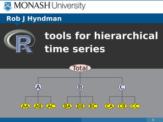
1. Total
A
AA AB AC
B
BA BB BC
C
CA CB CC
1
Rob J Hyndman
tools for hierarchical
time series

2. Introduction
Total
A
AA AB AC
B
BA BB BC
C
CA CB CC
Examples
Manufacturing product hierarchies
Pharmaceutical sales
Net labour turnover
hts: R tools for hierarchical time series 2

3. Introduction
Total
A
AA AB AC
B
BA BB BC
C
CA CB CC
Examples
Manufacturing product hierarchies
Pharmaceutical sales
Net labour turnover
hts: R tools for hierarchical time series 2

4. Introduction
Total
A
AA AB AC
B
BA BB BC
C
CA CB CC
Examples
Manufacturing product hierarchies
Pharmaceutical sales
Net labour turnover
hts: R tools for hierarchical time series 2

5. Introduction
Total
A
AA AB AC
B
BA BB BC
C
CA CB CC
Examples
Manufacturing product hierarchies
Pharmaceutical sales
Net labour turnover
hts: R tools for hierarchical time series 2

6. Hierarchical/grouped time series
A hierarchical time series is a collection of
several time series that are linked together in a
hierarchical structure.
Example: Pharmaceutical products are organized in
a hierarchy under the Anatomical Therapeutic
Chemical (ATC) Classification System.
A grouped time series is a collection of time
series that are aggregated in a number of
non-hierarchical ways.
Example: daily numbers of calls to HP call centres
are grouped by product type and location of call
centre.
hts: R tools for hierarchical time series 3

7. Hierarchical/grouped time series
A hierarchical time series is a collection of
several time series that are linked together in a
hierarchical structure.
Example: Pharmaceutical products are organized in
a hierarchy under the Anatomical Therapeutic
Chemical (ATC) Classification System.
A grouped time series is a collection of time
series that are aggregated in a number of
non-hierarchical ways.
Example: daily numbers of calls to HP call centres
are grouped by product type and location of call
centre.
hts: R tools for hierarchical time series 3

8. Hierarchical/grouped time series
A hierarchical time series is a collection of
several time series that are linked together in a
hierarchical structure.
Example: Pharmaceutical products are organized in
a hierarchy under the Anatomical Therapeutic
Chemical (ATC) Classification System.
A grouped time series is a collection of time
series that are aggregated in a number of
non-hierarchical ways.
Example: daily numbers of calls to HP call centres
are grouped by product type and location of call
centre.
hts: R tools for hierarchical time series 3

9. Hierarchical/grouped time series
A hierarchical time series is a collection of
several time series that are linked together in a
hierarchical structure.
Example: Pharmaceutical products are organized in
a hierarchy under the Anatomical Therapeutic
Chemical (ATC) Classification System.
A grouped time series is a collection of time
series that are aggregated in a number of
non-hierarchical ways.
Example: daily numbers of calls to HP call centres
are grouped by product type and location of call
centre.
hts: R tools for hierarchical time series 3

10. Hierarchical/grouped time series
Forecasts should be “aggregate
consistent”, unbiased, minimum variance.
Existing methods:
¢ Bottom-up
¢ Top-down
¢ Middle-out
How to compute forecast intervals?
Most research is concerned about relative
performance of existing methods.
There is no research on how to deal with
forecasting grouped time series.
hts: R tools for hierarchical time series 4

11. Hierarchical/grouped time series
Forecasts should be “aggregate
consistent”, unbiased, minimum variance.
Existing methods:
¢ Bottom-up
¢ Top-down
¢ Middle-out
How to compute forecast intervals?
Most research is concerned about relative
performance of existing methods.
There is no research on how to deal with
forecasting grouped time series.
hts: R tools for hierarchical time series 4

12. Hierarchical/grouped time series
Forecasts should be “aggregate
consistent”, unbiased, minimum variance.
Existing methods:
¢ Bottom-up
¢ Top-down
¢ Middle-out
How to compute forecast intervals?
Most research is concerned about relative
performance of existing methods.
There is no research on how to deal with
forecasting grouped time series.
hts: R tools for hierarchical time series 4

13. Hierarchical/grouped time series
Forecasts should be “aggregate
consistent”, unbiased, minimum variance.
Existing methods:
¢ Bottom-up
¢ Top-down
¢ Middle-out
How to compute forecast intervals?
Most research is concerned about relative
performance of existing methods.
There is no research on how to deal with
forecasting grouped time series.
hts: R tools for hierarchical time series 4

14. Hierarchical/grouped time series
Forecasts should be “aggregate
consistent”, unbiased, minimum variance.
Existing methods:
¢ Bottom-up
¢ Top-down
¢ Middle-out
How to compute forecast intervals?
Most research is concerned about relative
performance of existing methods.
There is no research on how to deal with
forecasting grouped time series.
hts: R tools for hierarchical time series 4

15. Hierarchical/grouped time series
Forecasts should be “aggregate
consistent”, unbiased, minimum variance.
Existing methods:
¢ Bottom-up
¢ Top-down
¢ Middle-out
How to compute forecast intervals?
Most research is concerned about relative
performance of existing methods.
There is no research on how to deal with
forecasting grouped time series.
hts: R tools for hierarchical time series 4

16. Hierarchical/grouped time series
Forecasts should be “aggregate
consistent”, unbiased, minimum variance.
Existing methods:
¢ Bottom-up
¢ Top-down
¢ Middle-out
How to compute forecast intervals?
Most research is concerned about relative
performance of existing methods.
There is no research on how to deal with
forecasting grouped time series.
hts: R tools for hierarchical time series 4

17. Hierarchical/grouped time series
Forecasts should be “aggregate
consistent”, unbiased, minimum variance.
Existing methods:
¢ Bottom-up
¢ Top-down
¢ Middle-out
How to compute forecast intervals?
Most research is concerned about relative
performance of existing methods.
There is no research on how to deal with
forecasting grouped time series.
hts: R tools for hierarchical time series 4

18. Hierarchical data
Total
A B C
hts: R tools for hierarchical time series 5
Yt : observed aggregate of all
series at time t.
YX,t : observation on series X at
time t.
Bt : vector of all series at
bottom level in time t.

19. Hierarchical data
Total
A B C
hts: R tools for hierarchical time series 5
Yt : observed aggregate of all
series at time t.
YX,t : observation on series X at
time t.
Bt : vector of all series at
bottom level in time t.

20. Hierarchical data
Total
A B C
Yt = [Yt, YA,t, YB,t, YC,t] =




1 1 1
1 0 0
0 1 0
0 0 1






YA,t
YB,t
YC,t


hts: R tools for hierarchical time series 5
Yt : observed aggregate of all
series at time t.
YX,t : observation on series X at
time t.
Bt : vector of all series at
bottom level in time t.

21. Hierarchical data
Total
A B C
Yt = [Yt, YA,t, YB,t, YC,t] =




1 1 1
1 0 0
0 1 0
0 0 1




S


YA,t
YB,t
YC,t


hts: R tools for hierarchical time series 5
Yt : observed aggregate of all
series at time t.
YX,t : observation on series X at
time t.
Bt : vector of all series at
bottom level in time t.

22. Hierarchical data
Total
A B C
Yt = [Yt, YA,t, YB,t, YC,t] =




1 1 1
1 0 0
0 1 0
0 0 1




S


YA,t
YB,t
YC,t


Bt
hts: R tools for hierarchical time series 5
Yt : observed aggregate of all
series at time t.
YX,t : observation on series X at
time t.
Bt : vector of all series at
bottom level in time t.

23. Hierarchical data
Total
A B C
Yt = [Yt, YA,t, YB,t, YC,t] =




1 1 1
1 0 0
0 1 0
0 0 1




S


YA,t
YB,t
YC,t


Bt
Yt = SBt
hts: R tools for hierarchical time series 5
Yt : observed aggregate of all
series at time t.
YX,t : observation on series X at
time t.
Bt : vector of all series at
bottom level in time t.

24. Hierarchical data
Total
A
AX AY AZ
B
BX BY BZ
C
CX CY CZ
Yt =












Yt
YA,t
YB,t
YC,t
YAX,t
YAY,t
YAZ,t
YBX,t
YBY,t
YBZ,t
YCX,t
YCY,t
YCZ,t












=












1 1 1 1 1 1 1 1 1
1 1 1 0 0 0 0 0 0
0 0 0 1 1 1 0 0 0
0 0 0 0 0 0 1 1 1
1 0 0 0 0 0 0 0 0
0 1 0 0 0 0 0 0 0
0 0 1 0 0 0 0 0 0
0 0 0 1 0 0 0 0 0
0 0 0 0 1 0 0 0 0
0 0 0 0 0 1 0 0 0
0 0 0 0 0 0 1 0 0
0 0 0 0 0 0 0 1 0
0 0 0 0 0 0 0 0 1












S







YAX,t
YAY,t
YAZ,t
YBX,t
YBY,t
YBZ,t
YCX,t
YCY,t
YCZ,t







Bt
hts: R tools for hierarchical time series 6

25. Hierarchical data
Total
A
AX AY AZ
B
BX BY BZ
C
CX CY CZ
Yt =












Yt
YA,t
YB,t
YC,t
YAX,t
YAY,t
YAZ,t
YBX,t
YBY,t
YBZ,t
YCX,t
YCY,t
YCZ,t












=












1 1 1 1 1 1 1 1 1
1 1 1 0 0 0 0 0 0
0 0 0 1 1 1 0 0 0
0 0 0 0 0 0 1 1 1
1 0 0 0 0 0 0 0 0
0 1 0 0 0 0 0 0 0
0 0 1 0 0 0 0 0 0
0 0 0 1 0 0 0 0 0
0 0 0 0 1 0 0 0 0
0 0 0 0 0 1 0 0 0
0 0 0 0 0 0 1 0 0
0 0 0 0 0 0 0 1 0
0 0 0 0 0 0 0 0 1












S







YAX,t
YAY,t
YAZ,t
YBX,t
YBY,t
YBZ,t
YCX,t
YCY,t
YCZ,t







Bt
hts: R tools for hierarchical time series 6

26. Hierarchical data
Total
A
AX AY AZ
B
BX BY BZ
C
CX CY CZ
Yt =












Yt
YA,t
YB,t
YC,t
YAX,t
YAY,t
YAZ,t
YBX,t
YBY,t
YBZ,t
YCX,t
YCY,t
YCZ,t












=












1 1 1 1 1 1 1 1 1
1 1 1 0 0 0 0 0 0
0 0 0 1 1 1 0 0 0
0 0 0 0 0 0 1 1 1
1 0 0 0 0 0 0 0 0
0 1 0 0 0 0 0 0 0
0 0 1 0 0 0 0 0 0
0 0 0 1 0 0 0 0 0
0 0 0 0 1 0 0 0 0
0 0 0 0 0 1 0 0 0
0 0 0 0 0 0 1 0 0
0 0 0 0 0 0 0 1 0
0 0 0 0 0 0 0 0 1












S







YAX,t
YAY,t
YAZ,t
YBX,t
YBY,t
YBZ,t
YCX,t
YCY,t
YCZ,t







Bt
hts: R tools for hierarchical time series 6
Yt = SBt

27. Grouped data
Total
A
AX AY
B
BX BY
Total
X
AX BX
Y
AY BY
Yt =













Yt
YA,t
YB,t
YX,t
YY,t
YAX,t
YAY,t
YBX,t
YBY,t













=













1 1 1 1
1 1 0 0
0 0 1 1
1 0 1 0
0 1 0 1
1 0 0 0
0 1 0 0
0 0 1 0
0 0 0 1













S



YAX,t
YAY,t
YBX,t
YBY,t



Bt
hts: R tools for hierarchical time series 7

28. Grouped data
Total
A
AX AY
B
BX BY
Total
X
AX BX
Y
AY BY
Yt =













Yt
YA,t
YB,t
YX,t
YY,t
YAX,t
YAY,t
YBX,t
YBY,t













=













1 1 1 1
1 1 0 0
0 0 1 1
1 0 1 0
0 1 0 1
1 0 0 0
0 1 0 0
0 0 1 0
0 0 0 1













S



YAX,t
YAY,t
YBX,t
YBY,t



Bt
hts: R tools for hierarchical time series 7

29. Grouped data
Total
A
AX AY
B
BX BY
Total
X
AX BX
Y
AY BY
Yt =













Yt
YA,t
YB,t
YX,t
YY,t
YAX,t
YAY,t
YBX,t
YBY,t













=













1 1 1 1
1 1 0 0
0 0 1 1
1 0 1 0
0 1 0 1
1 0 0 0
0 1 0 0
0 0 1 0
0 0 0 1













S



YAX,t
YAY,t
YBX,t
YBY,t



Bt
hts: R tools for hierarchical time series 7
Yt = SBt

30. Forecasts
Key idea: forecast reconciliation
¯ Ignore structural constraints and forecast
every series of interest independently.
¯ Adjust forecasts to impose constraints.
Let ˆYn(h) be vector of initial h-step forecasts,
made at time n, stacked in same order as Yt.
Yt = SBt . So ˆYn(h) = Sβn(h) + εh .
βn(h) = E[Bn+h | Y1, . . . , Yn].
εh has zero mean and covariance Σh.
Estimate βn(h) using GLS?
hts: R tools for hierarchical time series 8

31. Forecasts
Key idea: forecast reconciliation
¯ Ignore structural constraints and forecast
every series of interest independently.
¯ Adjust forecasts to impose constraints.
Let ˆYn(h) be vector of initial h-step forecasts,
made at time n, stacked in same order as Yt.
Yt = SBt . So ˆYn(h) = Sβn(h) + εh .
βn(h) = E[Bn+h | Y1, . . . , Yn].
εh has zero mean and covariance Σh.
Estimate βn(h) using GLS?
hts: R tools for hierarchical time series 8

32. Forecasts
Key idea: forecast reconciliation
¯ Ignore structural constraints and forecast
every series of interest independently.
¯ Adjust forecasts to impose constraints.
Let ˆYn(h) be vector of initial h-step forecasts,
made at time n, stacked in same order as Yt.
Yt = SBt . So ˆYn(h) = Sβn(h) + εh .
βn(h) = E[Bn+h | Y1, . . . , Yn].
εh has zero mean and covariance Σh.
Estimate βn(h) using GLS?
hts: R tools for hierarchical time series 8

33. Forecasts
Key idea: forecast reconciliation
¯ Ignore structural constraints and forecast
every series of interest independently.
¯ Adjust forecasts to impose constraints.
Let ˆYn(h) be vector of initial h-step forecasts,
made at time n, stacked in same order as Yt.
Yt = SBt . So ˆYn(h) = Sβn(h) + εh .
βn(h) = E[Bn+h | Y1, . . . , Yn].
εh has zero mean and covariance Σh.
Estimate βn(h) using GLS?
hts: R tools for hierarchical time series 8

34. Forecasts
Key idea: forecast reconciliation
¯ Ignore structural constraints and forecast
every series of interest independently.
¯ Adjust forecasts to impose constraints.
Let ˆYn(h) be vector of initial h-step forecasts,
made at time n, stacked in same order as Yt.
Yt = SBt . So ˆYn(h) = Sβn(h) + εh .
βn(h) = E[Bn+h | Y1, . . . , Yn].
εh has zero mean and covariance Σh.
Estimate βn(h) using GLS?
hts: R tools for hierarchical time series 8

35. Forecasts
Key idea: forecast reconciliation
¯ Ignore structural constraints and forecast
every series of interest independently.
¯ Adjust forecasts to impose constraints.
Let ˆYn(h) be vector of initial h-step forecasts,
made at time n, stacked in same order as Yt.
Yt = SBt . So ˆYn(h) = Sβn(h) + εh .
βn(h) = E[Bn+h | Y1, . . . , Yn].
εh has zero mean and covariance Σh.
Estimate βn(h) using GLS?
hts: R tools for hierarchical time series 8

36. Forecasts
Key idea: forecast reconciliation
¯ Ignore structural constraints and forecast
every series of interest independently.
¯ Adjust forecasts to impose constraints.
Let ˆYn(h) be vector of initial h-step forecasts,
made at time n, stacked in same order as Yt.
Yt = SBt . So ˆYn(h) = Sβn(h) + εh .
βn(h) = E[Bn+h | Y1, . . . , Yn].
εh has zero mean and covariance Σh.
Estimate βn(h) using GLS?
hts: R tools for hierarchical time series 8

37. Optimal combination forecasts
˜Yn(h) = S ˆβn(h) = S(S Σ†
hS)−1
S Σ†
h
ˆYn(h)
Σ†
h is generalized inverse of Σh.
Problem: Σh hard to estimate.
Solution: Assume εh ≈ SεK,h where εK,h is
the forecast error at bottom level.
Then Σh ≈ SΩhS where Ωh = Var(εK,h).
If Moore-Penrose generalized inverse used,
then (S Σ†
S)−1
S Σ†
= (S S)−1
S .
˜Yn(h) = S(S S)−1
S ˆYn(h)
hts: R tools for hierarchical time series 9

38. Optimal combination forecasts
˜Yn(h) = S ˆβn(h) = S(S Σ†
hS)−1
S Σ†
h
ˆYn(h)
Initial forecasts
Σ†
h is generalized inverse of Σh.
Problem: Σh hard to estimate.
Solution: Assume εh ≈ SεK,h where εK,h is
the forecast error at bottom level.
Then Σh ≈ SΩhS where Ωh = Var(εK,h).
If Moore-Penrose generalized inverse used,
then (S Σ†
S)−1
S Σ†
= (S S)−1
S .
˜Yn(h) = S(S S)−1
S ˆYn(h)
hts: R tools for hierarchical time series 9

39. Optimal combination forecasts
˜Yn(h) = S ˆβn(h) = S(S Σ†
hS)−1
S Σ†
h
ˆYn(h)
Revised forecasts Initial forecasts
Σ†
h is generalized inverse of Σh.
Problem: Σh hard to estimate.
Solution: Assume εh ≈ SεK,h where εK,h is
the forecast error at bottom level.
Then Σh ≈ SΩhS where Ωh = Var(εK,h).
If Moore-Penrose generalized inverse used,
then (S Σ†
S)−1
S Σ†
= (S S)−1
S .
˜Yn(h) = S(S S)−1
S ˆYn(h)
hts: R tools for hierarchical time series 9

40. Optimal combination forecasts
˜Yn(h) = S ˆβn(h) = S(S Σ†
hS)−1
S Σ†
h
ˆYn(h)
Revised forecasts Initial forecasts
Σ†
h is generalized inverse of Σh.
Problem: Σh hard to estimate.
Solution: Assume εh ≈ SεK,h where εK,h is
the forecast error at bottom level.
Then Σh ≈ SΩhS where Ωh = Var(εK,h).
If Moore-Penrose generalized inverse used,
then (S Σ†
S)−1
S Σ†
= (S S)−1
S .
˜Yn(h) = S(S S)−1
S ˆYn(h)
hts: R tools for hierarchical time series 9

41. Optimal combination forecasts
˜Yn(h) = S ˆβn(h) = S(S Σ†
hS)−1
S Σ†
h
ˆYn(h)
Revised forecasts Initial forecasts
Σ†
h is generalized inverse of Σh.
Problem: Σh hard to estimate.
Solution: Assume εh ≈ SεK,h where εK,h is
the forecast error at bottom level.
Then Σh ≈ SΩhS where Ωh = Var(εK,h).
If Moore-Penrose generalized inverse used,
then (S Σ†
S)−1
S Σ†
= (S S)−1
S .
˜Yn(h) = S(S S)−1
S ˆYn(h)
hts: R tools for hierarchical time series 9

42. Optimal combination forecasts
˜Yn(h) = S ˆβn(h) = S(S Σ†
hS)−1
S Σ†
h
ˆYn(h)
Revised forecasts Initial forecasts
Σ†
h is generalized inverse of Σh.
Problem: Σh hard to estimate.
Solution: Assume εh ≈ SεK,h where εK,h is
the forecast error at bottom level.
Then Σh ≈ SΩhS where Ωh = Var(εK,h).
If Moore-Penrose generalized inverse used,
then (S Σ†
S)−1
S Σ†
= (S S)−1
S .
˜Yn(h) = S(S S)−1
S ˆYn(h)
hts: R tools for hierarchical time series 9

43. Optimal combination forecasts
˜Yn(h) = S ˆβn(h) = S(S Σ†
hS)−1
S Σ†
h
ˆYn(h)
Revised forecasts Initial forecasts
Σ†
h is generalized inverse of Σh.
Problem: Σh hard to estimate.
Solution: Assume εh ≈ SεK,h where εK,h is
the forecast error at bottom level.
Then Σh ≈ SΩhS where Ωh = Var(εK,h).
If Moore-Penrose generalized inverse used,
then (S Σ†
S)−1
S Σ†
= (S S)−1
S .
˜Yn(h) = S(S S)−1
S ˆYn(h)
hts: R tools for hierarchical time series 9

44. Optimal combination forecasts
˜Yn(h) = S ˆβn(h) = S(S Σ†
hS)−1
S Σ†
h
ˆYn(h)
Revised forecasts Initial forecasts
Σ†
h is generalized inverse of Σh.
Problem: Σh hard to estimate.
Solution: Assume εh ≈ SεK,h where εK,h is
the forecast error at bottom level.
Then Σh ≈ SΩhS where Ωh = Var(εK,h).
If Moore-Penrose generalized inverse used,
then (S Σ†
S)−1
S Σ†
= (S S)−1
S .
˜Yn(h) = S(S S)−1
S ˆYn(h)
hts: R tools for hierarchical time series 9

45. Optimal combination forecasts
˜Yn(h) = S ˆβn(h) = S(S Σ†
hS)−1
S Σ†
h
ˆYn(h)
Revised forecasts Initial forecasts
Σ†
h is generalized inverse of Σh.
Problem: Σh hard to estimate.
Solution: Assume εh ≈ SεK,h where εK,h is
the forecast error at bottom level.
Then Σh ≈ SΩhS where Ωh = Var(εK,h).
If Moore-Penrose generalized inverse used,
then (S Σ†
S)−1
S Σ†
= (S S)−1
S .
˜Yn(h) = S(S S)−1
S ˆYn(h)
hts: R tools for hierarchical time series 9

46. Optimal combination forecasts
˜Yn(h) = S ˆβn(h) = S(S Σ†
hS)−1
S Σ†
h
ˆYn(h)
Revised forecasts Initial forecasts
Σ†
h is generalized inverse of Σh.
Problem: Σh hard to estimate.
Solution: Assume εh ≈ SεK,h where εK,h is
the forecast error at bottom level.
Then Σh ≈ SΩhS where Ωh = Var(εK,h).
If Moore-Penrose generalized inverse used,
then (S Σ†
S)−1
S Σ†
= (S S)−1
S .
˜Yn(h) = S(S S)−1
S ˆYn(h)
hts: R tools for hierarchical time series 9

47. Optimal combination forecasts
˜Yn(h) = S(S S)−1
S ˆYn(h)
GLS = OLS.
Optimal weighted average of initial
forecasts.
Optimal reconciliation weights are
S(S S)−1
S .
Weights are independent of the data and
of the covariance structure of the
hierarchy!
hts: R tools for hierarchical time series 10

48. Optimal combination forecasts
˜Yn(h) = S(S S)−1
S ˆYn(h)
GLS = OLS.
Optimal weighted average of initial
forecasts.
Optimal reconciliation weights are
S(S S)−1
S .
Weights are independent of the data and
of the covariance structure of the
hierarchy!
hts: R tools for hierarchical time series 10

49. Optimal combination forecasts
˜Yn(h) = S(S S)−1
S ˆYn(h)
GLS = OLS.
Optimal weighted average of initial
forecasts.
Optimal reconciliation weights are
S(S S)−1
S .
Weights are independent of the data and
of the covariance structure of the
hierarchy!
hts: R tools for hierarchical time series 10

50. Optimal combination forecasts
˜Yn(h) = S(S S)−1
S ˆYn(h)
GLS = OLS.
Optimal weighted average of initial
forecasts.
Optimal reconciliation weights are
S(S S)−1
S .
Weights are independent of the data and
of the covariance structure of the
hierarchy!
hts: R tools for hierarchical time series 10

51. Optimal combination forecasts
Total
A
AA AB AC
B
BA BB BC
C
CA CB CC
Weights: S(S S)−1
S =






















0.69 0.23 0.23 0.23 0.08 0.08 0.08 0.08 0.08 0.08 0.08 0.08 0.08
0.23 0.58 −0.17 −0.17 0.19 0.19 0.19 −0.06 −0.06 −0.06 −0.06 −0.06 −0.06
0.23 −0.17 0.58 −0.17 −0.06 −0.06 −0.06 0.19 0.19 0.19 −0.06 −0.06 −0.06
0.23 −0.17 −0.17 0.58 −0.06 −0.06 −0.06 −0.06 −0.06 −0.06 0.19 0.19 0.19
0.08 0.19 −0.06 −0.06 0.73 −0.27 −0.27 −0.02 −0.02 −0.02 −0.02 −0.02 −0.02
0.08 0.19 −0.06 −0.06 −0.27 0.73 −0.27 −0.02 −0.02 −0.02 −0.02 −0.02 −0.02
0.08 0.19 −0.06 −0.06 −0.27 −0.27 0.73 −0.02 −0.02 −0.02 −0.02 −0.02 −0.02
0.08 −0.06 0.19 −0.06 −0.02 −0.02 −0.02 0.73 −0.27 −0.27 −0.02 −0.02 −0.02
0.08 −0.06 0.19 −0.06 −0.02 −0.02 −0.02 −0.27 0.73 −0.27 −0.02 −0.02 −0.02
0.08 −0.06 0.19 −0.06 −0.02 −0.02 −0.02 −0.27 −0.27 0.73 −0.02 −0.02 −0.02
0.08 −0.06 −0.06 0.19 −0.02 −0.02 −0.02 −0.02 −0.02 −0.02 0.73 −0.27 −0.27
0.08 −0.06 −0.06 0.19 −0.02 −0.02 −0.02 −0.02 −0.02 −0.02 −0.27 0.73 −0.27
0.08 −0.06 −0.06 0.19 −0.02 −0.02 −0.02 −0.02 −0.02 −0.02 −0.27 −0.27 0.73






















hts: R tools for hierarchical time series 11

52. Optimal combination forecasts
Total
A
AA AB AC
B
BA BB BC
C
CA CB CC
Weights: S(S S)−1
S =






















0.69 0.23 0.23 0.23 0.08 0.08 0.08 0.08 0.08 0.08 0.08 0.08 0.08
0.23 0.58 −0.17 −0.17 0.19 0.19 0.19 −0.06 −0.06 −0.06 −0.06 −0.06 −0.06
0.23 −0.17 0.58 −0.17 −0.06 −0.06 −0.06 0.19 0.19 0.19 −0.06 −0.06 −0.06
0.23 −0.17 −0.17 0.58 −0.06 −0.06 −0.06 −0.06 −0.06 −0.06 0.19 0.19 0.19
0.08 0.19 −0.06 −0.06 0.73 −0.27 −0.27 −0.02 −0.02 −0.02 −0.02 −0.02 −0.02
0.08 0.19 −0.06 −0.06 −0.27 0.73 −0.27 −0.02 −0.02 −0.02 −0.02 −0.02 −0.02
0.08 0.19 −0.06 −0.06 −0.27 −0.27 0.73 −0.02 −0.02 −0.02 −0.02 −0.02 −0.02
0.08 −0.06 0.19 −0.06 −0.02 −0.02 −0.02 0.73 −0.27 −0.27 −0.02 −0.02 −0.02
0.08 −0.06 0.19 −0.06 −0.02 −0.02 −0.02 −0.27 0.73 −0.27 −0.02 −0.02 −0.02
0.08 −0.06 0.19 −0.06 −0.02 −0.02 −0.02 −0.27 −0.27 0.73 −0.02 −0.02 −0.02
0.08 −0.06 −0.06 0.19 −0.02 −0.02 −0.02 −0.02 −0.02 −0.02 0.73 −0.27 −0.27
0.08 −0.06 −0.06 0.19 −0.02 −0.02 −0.02 −0.02 −0.02 −0.02 −0.27 0.73 −0.27
0.08 −0.06 −0.06 0.19 −0.02 −0.02 −0.02 −0.02 −0.02 −0.02 −0.27 −0.27 0.73






















hts: R tools for hierarchical time series 11

53. Features
Forget “bottom up” or “top down”. This
approach combines all forecasts optimally.
Method outperforms bottom-up and
top-down, especially for middle levels.
Covariates can be included in initial forecasts.
Adjustments can be made to initial forecasts
at any level.
Very simple and flexible method. Can work
with any hierarchical or grouped time series.
Conceptually easy to implement: OLS on
base forecasts.
hts: R tools for hierarchical time series 12

54. Features
Forget “bottom up” or “top down”. This
approach combines all forecasts optimally.
Method outperforms bottom-up and
top-down, especially for middle levels.
Covariates can be included in initial forecasts.
Adjustments can be made to initial forecasts
at any level.
Very simple and flexible method. Can work
with any hierarchical or grouped time series.
Conceptually easy to implement: OLS on
base forecasts.
hts: R tools for hierarchical time series 12

55. Features
Forget “bottom up” or “top down”. This
approach combines all forecasts optimally.
Method outperforms bottom-up and
top-down, especially for middle levels.
Covariates can be included in initial forecasts.
Adjustments can be made to initial forecasts
at any level.
Very simple and flexible method. Can work
with any hierarchical or grouped time series.
Conceptually easy to implement: OLS on
base forecasts.
hts: R tools for hierarchical time series 12

56. Features
Forget “bottom up” or “top down”. This
approach combines all forecasts optimally.
Method outperforms bottom-up and
top-down, especially for middle levels.
Covariates can be included in initial forecasts.
Adjustments can be made to initial forecasts
at any level.
Very simple and flexible method. Can work
with any hierarchical or grouped time series.
Conceptually easy to implement: OLS on
base forecasts.
hts: R tools for hierarchical time series 12

57. Features
Forget “bottom up” or “top down”. This
approach combines all forecasts optimally.
Method outperforms bottom-up and
top-down, especially for middle levels.
Covariates can be included in initial forecasts.
Adjustments can be made to initial forecasts
at any level.
Very simple and flexible method. Can work
with any hierarchical or grouped time series.
Conceptually easy to implement: OLS on
base forecasts.
hts: R tools for hierarchical time series 12

58. Features
Forget “bottom up” or “top down”. This
approach combines all forecasts optimally.
Method outperforms bottom-up and
top-down, especially for middle levels.
Covariates can be included in initial forecasts.
Adjustments can be made to initial forecasts
at any level.
Very simple and flexible method. Can work
with any hierarchical or grouped time series.
Conceptually easy to implement: OLS on
base forecasts.
hts: R tools for hierarchical time series 12

59. Challenges
Computational difficulties in big
hierarchies due to size of the S matrix and
non-singular behavior of (S S).
Need to estimate covariance matrix to
produce prediction intervals.
hts: R tools for hierarchical time series 13

60. Challenges
Computational difficulties in big
hierarchies due to size of the S matrix and
non-singular behavior of (S S).
Need to estimate covariance matrix to
produce prediction intervals.
hts: R tools for hierarchical time series 13

61. hts package for R
hts: R tools for hierarchical time series 14
hts: Hierarchical and grouped time series
Methods for analysing and forecasting hierarchical and grouped
time series
Version: 3.01
Depends: forecast
Imports: SparseM
Published: 2013-05-07
Author: Rob J Hyndman, Roman A Ahmed, and Han Lin Shang
Maintainer: Rob J Hyndman <Rob.Hyndman at monash.edu>
License: GPL-2 | GPL-3 [expanded from: GPL (≥ 2)]

62. Example using R
library(hts)
# bts is a matrix containing the bottom level time series
# g describes the grouping/hierarchical structure
y <- hts(bts, g=c(1,1,2,2))
hts: R tools for hierarchical time series 15

63. Example using R
library(hts)
# bts is a matrix containing the bottom level time series
# g describes the grouping/hierarchical structure
y <- hts(bts, g=c(1,1,2,2))
hts: R tools for hierarchical time series 15
Total
A
AX AY
B
BX BY

64. Example using R
library(hts)
# bts is a matrix containing the bottom level time series
# g describes the grouping/hierarchical structure
y <- hts(bts, g=c(1,1,2,2))
# Forecast 10-step-ahead using optimal combination method
# ETS used for each series by default
fc <- forecast(y, h=10)
hts: R tools for hierarchical time series 16

65. Example using R
library(hts)
# bts is a matrix containing the bottom level time series
# g describes the grouping/hierarchical structure
y <- hts(bts, g=c(1,1,2,2))
# Forecast 10-step-ahead using optimal combination method
# ETS used for each series by default
fc <- forecast(y, h=10)
# Select your own methods
ally <- allts(y)
allf <- matrix(, nrow=10, ncol=ncol(ally))
for(i in 1:ncol(ally))
allf[,i] <- mymethod(ally[,i], h=10)
allf <- ts(allf, start=2004)
# Reconcile forecasts so they add up
fc2 <- combinef(allf, Smatrix(y))
hts: R tools for hierarchical time series 17

66. hts function
Usage
hts(y, g)
gts(y, g, hierarchical=FALSE)
Arguments
y Multivariate time series containing the bot-
tom level series
g Group matrix indicating the group structure,
with one column for each series when com-
pletely disaggregated, and one row for each
grouping of the time series.
hierarchical Indicates if the grouping matrix should be
treated as hierarchical.
Details
hts is simply a wrapper for gts(y,g,TRUE). Both return an
object of class gts.
hts: R tools for hierarchical time series 18

67. forecast.gts function
Usage
forecast(object, h,
method = c("comb", "bu", "mo", "tdgsf", "tdgsa", "tdfp", "all"),
fmethod = c("ets", "rw", "arima"), level, positive = FALSE,
xreg = NULL, newxreg = NULL, ...)
Arguments
object Hierarchical time series object of class gts.
h Forecast horizon
method Method for distributing forecasts within the hierarchy.
fmethod Forecasting method to use
level Level used for "middle-out" method (when method="mo")
positive If TRUE, forecasts are forced to be strictly positive
xreg When fmethod = "arima", a vector or matrix of external re-
gressors, which must have the same number of rows as the
original univariate time series
newxreg When fmethod = "arima", a vector or matrix of external re-
gressors, which must have the same number of rows as the
original univariate time series
... Other arguments passing to ets or auto.arima
hts: R tools for hierarchical time series 19

68. Utility functions
allts(y) Returns all series in the
hierarchy
Smatrix(y) Returns the summing matrix
combinef(f) Combines initial forecasts
optimally.
hts: R tools for hierarchical time series 20

69. More information
hts: R tools for hierarchical time series 21
Vignette on CRAN

70. References
RJ Hyndman, RA Ahmed, G Athanasopoulos, and
HL Shang (2011). “Optimal combination
forecasts for hierarchical time series”.
Computational Statistics and Data Analysis
55(9), 2579–2589
RJ Hyndman, RA Ahmed, and HL Shang (2013).
hts: Hierarchical time series.
cran.r-project.org/package=hts.
RJ Hyndman and G Athanasopoulos (2013).
Forecasting: principles and practice. OTexts.
OTexts.com/fpp/.
hts: R tools for hierarchical time series 22