SlideShare une entreprise Scribd logo
1  sur  41
Télécharger pour lire hors ligne
An Improved Method to Predict
Assignment of Stocks into Russell Indexes†
ITZHAK BEN-DAVID, FRANCESCO FRANZONI, and RABIH MOUSSAWI*
October 2019
ABSTRACT
A growing literature uses the Russell 1000/2000 reconstitution event as an identification strategy to
investigate corporate finance and asset pricing questions. To implement this identification strategy,
researchers need to approximate the ranking variable used to assign stocks to indexes. We develop
a procedure that predicts assignment to the Russell 1000/2000 with significant improvements
relative to previous approaches. We apply this methodology to extend the tests in Ben-David,
Franzoni, and Moussawi (2018).
Keywords: Russell, institutional investors, ETFs, volatility
JEL Classification: G12, G14, G15
†
This note follows the authors’ Journal of Finance publication. To reference this note, please cite:
(1) Ben-David, Itzhak, Francesco Franzoni, and Rabih Moussawi, 2018, Do ETFs Increase Volatility?, Journal of Finance 73(6),
2471–2535.
(2) Ben-David, Itzhak, Francesco Franzoni, and Rabih Moussawi, 2019, A Note to “Do ETFs Increase Volatility?”: An Improved
Method to Predict Assignment of Stocks into Russell Indexes, Journal of Finance Replications and Corrigenda (web-only:
https://afajof.org/comments-and-rejoinders/)
*
Ben-David is with the Fisher College of Business at The Ohio State University and the National Bureau of Economic Research;
Franzoni (corresponding author) is with USI Lugano, the Swiss Finance Institute, and the Center for Economic and Policy Research;
and Moussawi is with the Villanova School of Business, Villanova University, and Wharton Research Data Services, The Wharton
School at the University of Pennsylvania. We thank Jack Liebersohn and Fabrizio Mazzonna for helpful comments. The authors
do not have any material disclosure to make.
1
A growing empirical literature relies on the annual reconstitution of the Russell 1000/2000 indexes
to identify exogenous variation in index assignment, which in turn is used to explore a host of
research questions in corporate finance and asset pricing.1
A key input in this identification strategy
is the ranking that Russell uses for index assignment. Because this variable is proprietary,
researchers approximate it using publicly available data. In this paper, we provide a novel
methodology for predicting Russell’s assignment of stocks to the Russell 1000 and 2000 indexes
that results in lower assignment error than commonly used approaches.
The annual reconstitution of the Russell 1000/2000 indexes, which takes place in June,
relies on a mechanical rule that exploits the ranking of stocks by market capitalization in the month
of May (FTSE Russell (2019)). In the reconstitutions up to the year 2006, the 1,000 largest stocks
became members of the Russell 1000 on the reconstitution date, usually on the last trading day of
June, and the next 2,000 stocks became members of the Russell 2000.2
Because market
capitalization at the close of the last trading day of May is arguably a random variable outside of
companies’ control, the reconstitution event provides exogenous variation in index membership,
and hence researchers can use these events to study the impact of index membership on various
outcome variables. Moreover, the Russell 1000/2000 indexes are popular for benchmarking by
institutional investors. Stocks at the top of the Russell 2000 have a significantly larger weight in
1
Several scholars have used the annual reconstitution of the Russell 1000/2000 indexes to identify exogenous variation
in institutional ownership and its impact on various outcome variables in the domains of corporate finance and asset
pricing. For example, Chang, Hong, and Liskovich (2015) focus on stock prices following index reconstitution.
Mullins (2014) and Appel, Gormley, and Keim (2016, 2019a) study corporate governance. Schmidt and Fahlenbrach
(2017) focus on the effect of institutional investors and firm value. Boone and White (2015) study information
production given different environments of institutional investors. Fich, Harford, and Tran (2015) investigate the
effect of institutional investors’ monitoring in the context of acquisitions. Crane, Michenaud, and Weston (2016) study
institutional investors and payout policy. Bird and Karolyi (2016) relate institutional ownership to corporate disclosure
policy. Ben-David, Franzoni, and Moussawi (2018) explore the effects of ETFs on stock volatility.
2
See Appendix A for the exact rank dates and reconstitution dates from 1989 to 2019. After 2006, Russell introduced
a banding rule to limit the turnover of stocks in the indexes. The banding approach precludes the possibility of
implementing a fuzzy regression discontinuity design because it eliminates any meaningful variation around the cutoff
between the two indexes (see Appel, Gormley, and Keim (2019a, 2019b)).
2
the Russell 2000 index than stocks at the bottom of the Russell 1000. Thus, given the large amount
of assets under management (AUM) that are benchmarked to the Russell 2000 (Chang, Hong, and
Liskovich (2015)), the reconstitution generates large heterogeneity in indexed ownership across
the two sides of the cutoff for index assignment.
A hurdle in implementing this identification strategy is the fact that the market
capitalization that Russell uses to rank stocks in May is not publicly available. This variable does
not necessarily coincide with the standard measure of company market value in the finance
literature (i.e., the product of publicly traded shares and the market price based on data from the
Center for Research in Security Prices (CRSP)). In particular, Russell combines different issues of
the same company and includes nonpublicly traded shares when computing company market value
(FTSE Russell (2019)). Because Russell does not publish its ranking variable, researchers rely on
imperfect proxies to predict the assignment of stocks into the two indexes at reconstitution.
Getting closer to the true ranking variable that Russell uses is important for all researchers
using the Russell reconstitution event for identification. Irrespective of whether this identification
strategy is used in a regression discontinuity design (RDD), as in Wei and Young (2017) and
Glossner (2019), among others, or in an instrumental variable (IV) approach, as in Appel,
Gormley, and Keim (2016, 2019a), among others, the ranking variable that Russell uses in
assigning stocks to indexes is a key input in the regressions. The principal role of this unobservable
variable, therefore, motivates us to improve the approximation of the market capitalization that
Russell uses for index assignment.
We proceed as follows. In Section I, we briefly summarize the main issue in implementing
the fuzzy RDD for the Russell indexes. In particular, the commonly used methodology is based on
predicting assignment into the Russell indexes based on CRSP market capitalization. However,
3
this procedure results in significant misassignment, as shown by Appel, Gormley, and Keim
(2019b), which could lead to a weak first stage in the fuzzy RDD procedure. In Section II, we
show that the predicted assignment can be materially improved based on publicly available
information. Our method constructs a new market capitalization ranking that builds on public data
sources and closely follows the Russell methodology (FTSE Russell (2019)). We show in Section
III that this exercise generates a better approximation of the actual market capitalization that
Russell uses to determine index assignment than simpler procedures that rely solely on CRSP
market capitalization in May prior to reconstitution. We describe the construction procedure in
detail and make the data available to other researchers along with its code.
Finally, in Section III, we use this new ranking variable in a fuzzy RDD framework to extend and
corroborate the analysis in Ben-David, Franzoni, and Moussawi (2018). Section IV concludes.
I. Russell 1000/2000 Reconstitution within a Fuzzy RDD Framework
To demonstrate the use of the ranking variable in an econometric analysis, we consider the
fuzzy RDD procedure advocated by Wei and Young (2017) and Glossner (2019) for exploiting the
Russell reconstitution for empirical investigation. Because the actual running variable (market
capitalization ranking by Russell) is unobservable, a fuzzy RDD is a suitable approach as it
involves approximating the unobservable running variable with another variable.
The fuzzy RDD consists of a two-stage procedure (see, for example, Lee and Lemieux
(2010), Roberts and Whited (2013)). In the first stage, the actual treatment indicator is regressed
on the predicted treatment 𝜏, controls for polynomials of the fuzzy ranking variable 𝑅𝑎𝑛𝑘 , (that
is, the proxy for the unobservable ranking variable), and the interactions between the controls and
the predicted treatment to allow the polynomial to differ on the two sides of the cutoff:
4
𝑅2000 , 𝛼 𝛼 𝜏 , 𝛼 , 𝑅𝑎𝑛𝑘 , 𝛼 , 𝜏 , 𝑅𝑎𝑛𝑘 , 𝜈 , ,
(1)
where 𝑅2000 , is an indicator variable equal to one if the stock is assigned to the Russell 2000
(i.e., treated) and to zero if it is assigned to the Russell 1000 index, and 𝜏 , is an indicator equal to
one if 𝑅𝑎𝑛𝑘 , 0 and to zero otherwise.
In the second stage, the outcome variable of interest is regressed on the instrumented actual
treatment, controlling for the fuzzy assignment variable and its polynomials:
𝑌, 𝛽 𝛽 𝑅2000 , 𝛽 , 𝑅𝑎𝑛𝑘 , 𝛽 , 𝑅2000 , 𝑅𝑎𝑛𝑘 , 𝜀 , . 3
(2)
Prior literature proposes two approaches to approximate Russell’s ranking variable. One
approach bases rankings on weights in the Russell indexes in June. However, the weights are based
on float-adjusted market capitalization, and thus they differ from the original ranking variable,
which is not float-adjusted. Moreover, for this proxy to be valid in an RDD context, one has to
assume that variation in market capitalization between the end of May and the end of June is
negligible and independent of index assignment. This assumption appears unwarranted.
Reiterating a claim in Chang, Hong, and Liskovich (2015, p. 222), Wei and Young (2017) argue
that using end-of-June weights to construct a proxy for the original ranking variable generates
selection bias. Indeed, these authors show that some relevant variables (including institutional
ownership itself) display a pre-existing discontinuity at the cutoff when the June rankings are used
(for more details, see also Appel, Gormley, and Keim (2019b)).
3
In the literature, we find slightly different specifications of equation (2). Lee and Lemieux (2010) and Roberts and
Whited (2013) use ∑ 𝛽 , 𝜏 , 𝑅𝑎𝑛𝑘 , rather than ∑ 𝛽 , 𝑅2000 , 𝑅𝑎𝑛𝑘 , , whereas the specification that
we propose in equation (2) corresponds to equation (2) in Wei and Young (2017). In the tests below, we try both
specifications and the estimates are virtually identical.
5
A second approach uses CRSP market capitalization in May, prior to reconstitution, as a
ranking variable. This approach is more appropriate as it avoids the look-ahead bias embedded in
the first approach, as discussed in Wei and Young (2017).4
We add to these previous approaches by developing a new ranking variable with an
improved ability to predict index assignment, which makes fuzzy RDD feasible even in the
neighborhood of the cutoff. We discuss this variable and its construction next.
II. An Improved Ranking Variable
A. Data and Variable Construction
Russell ranks stocks based on their total market capitalization and uses the rankings to
assign stocks to the Russell 1000 and Russell 2000 indexes. Russell does not provide the ranking
data that it uses to determine index membership in May of each year. Russell began providing the
total market capitalization data on which ranking is constructed in 2012, several years after the
introduction of the banding rule in 2007.5
The market capitalization used by Russell differs from
what researchers usually construct as the product of shares outstanding in CRSP at the PERMNO
level and the stock price at the end of May. In what follows, we describe how we account for part
of this difference.
According to the detailed Russell U.S. 1000/2000 index reconstitution methodology (FTSE
Russell (2019)), two dates are relevant. The first is the “rank date,” when all eligible securities are
ranked by their total market capitalization and index membership is determined. The rank date was
4
The approaches in Chang, Hong, and Liskovich (2015), Wei and Young (2017), and Glossner (2018) also avoid
look-ahead bias by combining CRSP and Compustat and obtain significant predictive power around the cutoff.
5
Mullins (2014) and Appel, Gormley, and Keim (2016) obtain market capitalization data for some of the pre-banding
years from Russell. However, both conclude that these data lead to a very noisy proxy for the true variable used by
Russell.
6
the final trading day of May until 2015, when it was changed to a day in mid-May. Second, the
“reconstitution date” is the effective date of the reconstitution, which has been performed annually
since 1989. The annual reconstitution date was the final business day of June until 2004, when it
was revised to the last Friday in June. In 2007, along with the new banding methodology, an
exception was made to this rule: reconstitution was effective after the close on the last Friday in
June unless the last Friday occurs on the 28th, 29th, or 30th (see the table in Appendix A for exact
rank and reconstitution dates between 1989 and 2019).
On the rank date, the total market capitalization (nonfloat-adjusted) of all share classes is
used to determine index membership. On the reconstitution date, security membership in each
index becomes effective, and the weight of each security in each index is proportional to the float-
adjusted issue-specific market capitalization that Russell computes for each security.
Section 5 of the Russell documentation (FTSE Russell (2019)) provides details on the
criteria for inclusion in the U.S. Russell indexes. To be included in the index, Russell imposes
restrictions regarding listing location and incorporation status and also imposes trading criteria
(e.g., minimum closing price of $1, minimum total market capitalization of $30 million, minimum
voting requirements, and minimum available shares or a float of 5%). Russell excludes preferred
and convertible preferred stocks, redeemable shares, participating preferred stocks, warrants,
rights, depositary receipts, installment receipts, and trust receipts.
Section 6 of the Russell documentation provides details on the computation of each
company’s total market capitalization on the rank date. The nonfloat-adjusted total market
capitalization is constructed as the sum of the products of total shares outstanding across all share
classes at the company level times the market price at the close of the rank day in May. Section
6.2 gives details on the classes of common shares included in the computation of total market
7
capitalization: all common stock share classes of nonrestricted exchangeable shares and
partnership units/membership interests are included, while preferred stocks, convertible preferred
stocks, redeemable shares, and other preferred stocks, warrants, rights, installment receipts, and
trust receipts are excluded from the total market capitalization calculation.6
Starting with the universe of the Russell 3000 stocks, we proceed in several steps. We
explain these steps and their corresponding assumptions in detail below. Our methodology and
assumptions are also reflected in the code in Appendix B.
CRSP and Compustat are our main sources of information. We match each Russell
constituent to its CRSP PERMNO using historical CUSIP information in CRSP MSENAMES and
to Compustat’s GVKEY using Compustat Snapshot’s CNSECURITY datasets.
We rely on the CRSP database for information on reliable prices and shares outstanding
for all securities traded on a major exchange (variable PERMNO), as CRSP provides reliable
information on these measures for public stocks. We also use CRSP’s mapping of the different
issues to their company identifier (variable PERMCO), which we employ to compute our proxy
for Russell’s total market capitalization. In a few cases, Russell’s mapping of issues to companies
differs from CRSP’s, but we do not correct these cases to adhere to a rule-based method and avoid
ad hoc choices.7,8
6
Starting in 2005, IPOs are also added on a quarterly basis. Section 6.7 in FTSE Russell (2019) provides the details.
Because the empirical analysis focuses on the annual reconstitution in June, these details are less relevant here.
7
Among the cases in which Russell differs from CRSP in mapping issues to parent companies is TreeHouse Foods,
THS, with CUSIP 89469A10 and PERMNO 90775, which spun off from Dean Foods (PERMCO 14527) in 2005 and
was assigned a PERMCO of 46889 by CRSP. Russell, however, seems to combine the market capitalization of both
entities, which could explain THS being assigned to the Russell 1000 in June 2005. THS was reassigned to the Russell
2000 the following year. Lanier Worldwide (CUSIP 51589L10), which spun off from its parent Harris Corporation
(CUSIP 41387510) in 1999, is another example.
8
One could be tempted to reverse-engineer the difference between the ranking resulting from our methodology and
Russell’s assignments to infer the mapping of misclassified cases to share issuers and achieve full replication of
Russell assignments. However, the fact that these ex-post inferences would be made only for the few misclassified
8
We next turn to Compustat for information on common shares of stocks that are traded
over-the-counter (OTC), nonpublicly traded stocks, and securities that are not in CRSP. For
companies that have one or more of their share classes listed in OTC markets, and for three
companies that are not in the CRSP database,9
we use the Compustat Securities Daily database to
aggregate the market capitalization of the multiple issues (variable GVKEY-IID) at the company
level (variable GVKEY). For companies that have multiple shares of common stock where one or
more of these share classes is closely held and not publicly traded, we use the aggregated shares
outstanding variable in Compustat Quarterly for the nearest quarter (variable CSHOQ), which
represents the total number of all common shares outstanding at fiscal quarter-end collected from
Forms 10-Q and 10-K.
After carving out the proportion of CSHOQ attributable to nontraded share classes, we
multiply it by the weighted-by-share-class-size average price of publicly traded share classes to
compute the corresponding market capitalization.10
We then add the market capitalization of the
closely held share classes to the market capitalization of the traded share classes computed using
Compustat to obtain a second proxy for the total market capitalization used by Russell in ranking
stocks.
In sum, we end up with two proxies for total market capitalization at the company level.
We rely primarily on the CRSP-based proxy for total market capitalization. We use the Compustat-
based proxy for total market capitalization only if it is higher than the CRSP-based figure.
cases would give no guarantee that the researcher has fully replicated Russell’s methodology, in which case the
resulting ranking of companies would not necessarily be superior to the rule-based approach that we follow.
9
CUSIPs: 03957A10, 26187710, and 71343P10.
10
Because closely held share classes are likely to have superior voting or cash flow rights, one might argue that it
would be more appropriate to use the highest price in computing the market capitalization for those nontraded shares.
Using this approach leads to very similar ranking outcomes and does not change the statistical or economic
significance of the empirical findings in our RDD tests.
9
B. Assessment of the Improvement in Index Assignment
The new ranking variable improves the predicted assignment: the new variable has a 99.7%
success rate in predicting index assignments between Russell 1000 and Russell 2000. Table I
provides descriptive statistics on the new variable’s performance. Panel A compares the market
capitalization obtained using the new ranking variable to that based on other measures.11
The panel
shows that our variable almost always generates a higher estimate of market capitalization. For the
first three alternative measures of market capitalization, 75% to 80% of stocks’ market
capitalization is virtually the same (up to 0.1% deviation) as the estimate obtained using our
variable. Only 5% to 7% of stocks’ market capitalization generate deviations that are greater than
10%. Our new variable is closest to the total market capitalization obtained using Compustat
Quarterly shares outstanding (CSHOQ), with the estimates overlapping completely for 95% of the
firm-years. The deviations for the remaining 5% are mostly smaller than 1%. Nevertheless, as we
show in the discussion of Table II below, large differences in a few firms result in weaker
econometric performance.
--- Table I goes about here ---
Table I, Panel B compares the performance of our rank variable to that of rank variables
used in prior literature that are based primarily on CRSP market capitalization or other viable
alternatives based on Compustat. Our rank variable leads to a total of 61 misclassified assignments
to the Russell 1000 and Russell 2000 during reconstitution over our sample period (i.e., 2000 to
2006). The CRSP- and Compustat-only rank variables produce many more misclassifications and
11
The other variables in the comparison are total market capitalization using CRSP at the issue level (PERMNO),
total market capitalization using CRSP aggregated at the company level (PERMCO), total market capitalization using
the Compustat Securities Daily database aggregated at the company level (GVKEY), and total market capitalization
using Compustat Quarterly shares outstanding (CSHOQ).
10
are inferior to our rank variable in each of the reconstitution years in our sample. We use the rank
variable obtained from our reconstructed market capitalization directly in our regression
discontinuity analysis.
We investigate further to better understand the reason for the few remaining discrepancies
between the Russell index assignments and those based on our rank variable. We notice that in a
few cases, Russell considers each class of stock separately, mainly when Russell believes that the
common stock share classes act independently of one another. In these cases, Russell differs from
CRSP in the issue-company aggregation, as Russell uses issue-level market capitalization instead
of total company-level market capitalization in determining index membership. For example, in a
few instances, stocks assigned to the Russell 2000 have company-level market capitalization
suggesting a Russell 1000 assignment but issue-level market capitalization suggesting a Russell
2000 assignment. In a few other cases, primarily related to recent spinoffs, Russell aggregates the
market cap of the parent and spun-off entities and ranks both entities as one. These cases do not
seem to follow a systematic pattern, so we cannot infer a rule-based systematic approach to account
for them.
To study the power of this new ranking variable in predicting index assignment, we run
regressions based on equation (1). Following the recommendation in Lee and Lemieux (2010), in
Figure 1 we start by plotting the treatment probability (that is, the probability of membership in
the Russell 2000 after reconstitution) as a function of the ranking variable. The clear discontinuity
at zero testifies to the success of our ranking methodology in closely approximating Russell’s
assignment approach.12
12
For graphical convenience, the variable 𝑅𝑎𝑛𝑘 , has been centered on the 1,000th position in terms of market
capitalization. Hence, 𝑅𝑎𝑛𝑘 , 0 corresponds to stocks predicted to end up in the Russell 2000, and 𝑅𝑎𝑛𝑘 , 0
corresponds to stocks predicted to end up in the Russell 1000.
11
--- Figure 1 goes about here ---
We next report results of the regression analyses in Panel A of Table II.13
The dependent
variable is an indicator for whether the stock is assigned to the Russell 2000 in the reconstitution
event. The main variable of interest, 𝜏, is a dummy variable that indicates whether our market
capitalization variable is above 1,000. We report regressions for four different bandwidths (50,
100, 200, and 400) and specifications including polynomials of the first, second, and third degree.
The results show that our ranking variable has statistically strong predictive power for the
assignment probability in 11 out of the 12 regressions. The only regression with no statistical
significance is that with a bandwidth of ±50 and a third-order polynomial (column (3)). The lack
of significance in this specification is arguably due to the fact that the degree of the polynomial is
too high for the small number of observations.
This analysis also allows us to benchmark our approach against those used by other
researchers. We note, however, that our analysis is conducted on somewhat different sample
periods from those in other papers, and thus coefficients are not fully comparable. Wei and Young
(2017) use a bandwidth of 100 with a linear specification (Table 5, column (2) in their paper).
They find a coefficient of 0.72. In the same specification, we obtain an estimate of 0.82 (our Table
II, Panel A, column (4)). In a specification with a bandwidth of 200 and a third-order polynomial
(their column (1)), their coefficient is 0.55, whereas the corresponding coefficient for us is 0.69
(our Table II, Panel A, column (9)). When we apply Wei and Young’s (2017) procedure to our
sample period (2000 to 2006), the estimates are not distinguishable from ours. Appel, Gormley,
and Keim (2019b; their Table 2) use bandwidths of 50 and 100 with polynomials of the first to
13
The two-stage least squares estimation includes additional first-stage regressions in which the dependent variables
are the assignment variable interacted with 𝑅𝑎𝑛𝑘𝑖,𝑡 and its polynomials. We do not report these regressions to save
space because they do not add relevant information.
12
third order. In that paper, five out of the six coefficients are statistically significant and negative.
In our Table II, Panel A, columns (1) to (6), all coefficients are positive and five out of the six are
statistically significant. Appel, Gormley, and Keim (2019b) also use a bandwidth of 250 and find
statistically significant coefficients ranging between 0.09 to 0.65. We use a slightly smaller
bandwidth of 200, and the coefficients range between 0.69 and 0.91.
--- Table II goes about here ---
We further compare the performance of our ranking variable to other candidates based on
simply using CRSP or Compustat market capitalization. In Table II, Panel B, we estimate equation
(1) for different bandwidths with rankings based on CRSP at the issue and company levels, as well
as on Compustat at the issue and company levels. The best-performing of these alternative ranking
variables seems to be that based on Compustat at the company level, consistent with the evidence
in Table I, Panel B on the number of misclassifications. However, the performance of this
alternative ranking variable in predicting assignment is still inferior to that of our ranking variable
in Panel A of Table II. The other variables perform even worse. For bandwidths of ±50 or ±100,
most of the slopes on 𝜏 are either statistically insignificant or significant but negative. For
bandwidths of ±200, the coefficients on the first- and second-degree polynomials are positive, but
their magnitude is relatively low. For bandwidths of ±400, all of the coefficients are positive, but
the magnitudes are always smaller than the magnitude of the corresponding regression in Panel A.
Overall, the coefficients in the regressions in Panel A are larger than the coefficients in each of the
corresponding regressions (same bandwidth and polynomial order) in Panel B.
To summarize, an assessment of the performance of our ranking variable shows that our
measure of total market capitalization has at least comparable and often superior performance in
predicting the Russell assignment than that of other viable candidates. Therefore, our variable can
13
help improve the significance of future studies that rely on Russell index assignments for
identification.
III. An Empirical Application of the New Ranking Variable
Ben-David, Franzoni, and Moussawi (2018) use the reconstitution of the Russell 1000/2000
indexes to identify exogenous variation in ETF ownership. The idea is that because most ETFs
passively track indexes, a mechanical and unanticipated change in index composition triggers
exogenous changes in ETF ownership at the stock level. In that paper, we use CRSP market
capitalization in May as a control variable, and thus our methodology is not exposed to the
criticism that June market capitalization rankings have attracted (Wei and Young (2017), Appel,
Gormley, and Keim (2019b), Glossner (2019)). Overall, the procedure closely follows prior
literature that also relies on the Russell reconstitution event (e.g., Appel, Gormley, and Keim
(2016)).
In this paper, we apply the newly created ranking variable to extend the analysis in Ben-
David, Franzoni, and Moussawi (2018) within the framework of a fuzzy RDD. Before doing so,
we briefly summarize the methodology that we adopt in the 2018 paper.
A. The Approach in Ben-David, Franzoni, and Moussawi (2018)
In Ben-David, Franzoni, and Moussawi (2018), we carry out a two-stage least squares
estimation. The first stage consists of a regression of ETF ownership on an indicator for whether
the stock switched index membership in June. For the Russell 1000 sample, the indicator variable
flags stocks that switched to the Russell 2000; for the Russell 2000 sample, the dummy captures a
switch to the Russell 1000. In regression form, the first stage is given by equation (4) in the original
paper. In the second stage, we regress daily volatility (computed using daily returns within the
14
month) on the fitted value of ETF ownership at the beginning of the month from the first stage.
This regression is given by equation (5) in the original paper.
We apply this approach to two separate samples that include stock-month observations
between June 2000 and May 2007, that is, all of the months following the annual reconstitutions
between 2000 and 2006. The first sample comprises all stocks that were in the Russell 1000 as of
May of each year, that is, prior to index reconstitution. The second sample comprises all stocks
that were in the Russell 2000 as of May. The sample composition is constant for all months
between June (the first month after index reconstitution) and May of the following year. The idea
underlying the tests is to compare the outcome variables (i.e., volatility) for stocks that changed
indexes versus stocks that remained in the same index, in a neighborhood of the cutoff for index
switching. Following common practice in the literature, we experiment with various bandwidths
around the cutoff (i.e., 50, 100, 200, and 400).
To address the concern that index switching is not an exogenous event relative to the
dependent variable of interest, we draw inspiration from the RDD methodology. In an RDD,
assignment to the treatment group is conditionally exogenous when the econometrician can control
for polynomials of the assignment variable. Because the actual Russell rankings in May are not
available, we use CRSP market capitalization rankings in May as a proxy. Hence, in our
specifications, we control for polynomials of the CRSP May market capitalization rankings to
make the treatment variable conditionally exogenous.
Additionally, one may be concerned that persistence in volatility could hardwire our
results. According to this argument, if lagged volatility increases the probability of switching
indexes and volatility is persistent, stocks that switch indexes may display higher future volatility.
However, this argument cannot explain why we find that stocks that switch from the Russell 2000
15
to the Russell 1000 display lower volatility (see Table V in the original article, columns (6) to
(10)). Moreover, this concern should not arise in the first place because we control for lagged
volatility in all of our specifications.
B. A Fuzzy RDD to Study the Impact of ETFs on Stock Volatility
In what follows, we use the newly created ranking variable within a fuzzy RDD to study
the impact of ETF ownership on stock volatility. We refer the reader to the original paper for the
motivation behind this analysis.
We assume that index redefinition affects stock volatility through ETF ownership. Hence,
to study the relation of interest, we can just use volatility as a dependent variable in equation (2).
However, because we also wish to express the estimates as a relation between volatility and ETF
ownership, we proceed with two-stage least squares estimation. The first stage is a reduced form
that combines equations (1) and (2). Specifically, we regress ETF ownership on the variable 𝜏 ,
and polynomials of the ranking variable:
𝐸𝑇𝐹𝑜𝑤𝑛 , 𝛿 𝛿 𝜏 , 𝛿 , 𝑅𝑎𝑛𝑘 , 𝛿 , 𝜏 , 𝑅𝑎𝑛𝑘 , 𝜖 , .
(3)
In the second stage, we regress daily volatility computed in the year after reconstitution on
instrumented ETF ownership in the December after reconstitution and polynomials of the ranking
variable:
𝑉𝑜𝑙𝑎𝑡𝑖𝑙𝑖𝑡𝑦 , 𝛾 𝛾 𝐸𝑇𝐹𝑜𝑤𝑛 , 𝛾 , 𝑅𝑎𝑛𝑘 , 𝛾 , 𝜏 , 𝑅𝑎𝑛𝑘 , 𝜔 , ,
(4)
16
where the coefficient 𝛾 measures the impact of an expected change in ETF ownership due to index
reconstitution, measured in standard deviation units, on stock return volatility after reconstitution,
also measured in standard deviation units.
In this analysis, we use one observation per stock-year and pool Russell 1000 and 2000
stocks together. The sample period coincides with the reconstitutions between 2000 and 2006,
before the banding rule was introduced. ETF ownership is measured at the end of December after
reconstitution, and volatility is measured from daily returns in the year after reconstitution.
Variable definitions and summary statistics are presented in Appendix C.
Before conducting the regression analysis, we provide a graphical summary of the data.14
Figure 2, Panel A presents ETF ownership (as of the December after reconstitution). ETF
ownership is expected to be significantly higher by about 40 bps for stocks predicted to end up in
the Russell 2000, that is, for rankings above zero, than for those predicted to enter the Russell
1000. The mean of ETF ownership in this sample is about 90 bps and the standard deviation is 84
bps. Hence, the increase is economically significant. When we use lagged ETF ownership in March
before reconstitution (Figure 2, Panel B), there is no discontinuity around the cutoff.
--- Figure 2 goes about here ---
In Figure 3, Panels A and B, we repeat the exercise for total institutional ownership net of
ETF ownership. Consistent with prior literature (e.g., Wei and Young (2017)), the panels show
that there is no positive jump in total institutional ownership net of ETFs in either the current year
or the preceding year. Hence, we conclude that the Russell reconstitution generates significant
changes in ETF ownership but not in institutional ownership in general.
14
Based on the argument in Gelman and Imbens (2019) that high-order polynomials lead to noisy estimates, in the
graphs we plot linear polynomials estimated with a triangular kernel centered on the cutoff.
17
--- Figure 3 goes about here ---
Finally, we present volatility and lagged volatility in Figure 4, Panels A and B. Here,
volatility is higher to the right of the cutoff, that is, for stocks that are predicted to end up in the
Russell 2000. We again find no visible discontinuity in volatility around the cutoff in the year
before the reconstitution event.
We next examine the relations of interest in a regression framework. Following equations
(1) and (2), we regress ETF ownership measured in the December after reconstitution on the
instrumented index assignment indicator. Table II, Panel A presents the results of the first-stage
regressions (predicting index assignment). We choose bandwidths around the cutoff ranging from
50 to 400 and present specifications with polynomials ranging from the first to the third order. The
regressions include time fixed effects to account for trends in ETF ownership, and we cluster
standard errors at the stock level.
Table III, Panel A presents results for the second stage on the level of ETF ownership in
December, which we standardize by dividing by the standard deviation in the regression sample.
The estimates show that ETF ownership is significantly higher for the largest stocks in the Russell
2000 relative to the smallest stocks in the Russell 1000, by 52% to 96% (depending on the
bandwidth and polynomial degree) of a standard deviation of the dependent variable. Hence, index
assignment generates a large change in ETF ownership, consistent with Figure 2, Panel A (in which
ETF ownership is not standardized).
--- Table III goes about here ---
Finally, Panel B of Table III uses the (standardized) change in ETF ownership between
March before reconstitution and December after reconstitution as the dependent variable. This
specification addresses the concern that there could be pre-determined differences in ETF
18
ownership around the cutoff. (Panel B of Figure 2 already helps rule out this possibility.) We notice
that (instrumented) assignment to treatment corresponds to large changes (of about one standard
deviation) in ETF ownership after reconstitution.
Table IV, Panel A reports the estimates of equation (4). We control for volatility in the
prior year to address the above-mentioned concern that volatility could affect the probability of
switching indexes. Across specifications, we find that volatility increases significantly with ETF
ownership, by 21% to 76% (depending on the bandwidth and polynomial degree) of a standard
deviation for a one-standard-deviation change in ETF ownership. Restricting attention to the
bandwidths above 50 for comparability, the magnitude of the median estimate is about 31%, which
is almost identical to the result presented in our 2018 paper of about 31% of a standard deviation.
--- Table IV goes about here ---
In Table IV, Panel B, we modify the specifications from Panel A so that the dependent
variable is the year-over-year change in daily volatility around the reconstitution date. In this case,
we do not include prior-year volatility among the controls. The estimates are consistent with Panel
A and show that volatility increases when ETF ownership rises as a consequence of index
reconstitution.
We next run regressions in which volatility is the dependent variable in equation (2) and
report the results in Table IV, Panel C. The estimates are again significant. Across specifications,
volatility is about 20% of a standard deviation higher for stocks in the Russell 2000 than for stocks
in the Russell 1000. We present the daily volatility as well as a linear fit in Figure 4, Panel A (in
which volatility is not standardized).
Gelman and Imbens (2019) argue that controlling for global high-order polynomials in
regression discontinuity analyses is a flawed approach because of noisy estimates, sensitivity to
19
the degree of the polynomial, and poor coverage of confidence intervals. They recommend instead
using estimators based on local linear or quadratic polynomials. Following their advice, in Table
IV, Panel D we modify the specifications of Panel C by including local polynomials of the first
and second degree. The results are virtually unchanged in terms of both magnitude and
significance.15
To conclude, the fuzzy RDD confirms the results in our 2018 article in terms of both
significance and magnitude.
IV. Conclusion
In this paper we provide an improved methodology for approximating the ranking variable
used by Russell to assign stocks to the Russell 1000/2000 indexes. The new ranking variable
produces a lower number of misclassified companies relative to other reasonable candidates and a
better prediction of the assignment probability than prior studies. Using this variable, we extend
and corroborate the findings in Ben-David, Franzoni, and Moussawi (2018).
We provide the code for constructing this variable in Appendix B of this paper. The data
are available to other researchers wishing to apply this identification strategy per request.
Initial submission: June 17, 2019; Accepted: September 6, 2019
Editors: Stefan Nagel, Philip Bond, Amit Seru, and Wei Xiong
15
Specifically, to carry out this estimation, we use the Stata-implemented command –rdrobust– (see Calonico et al.
(2017)) with a triangular kernel, clustering standard errors by stock. We include lagged volatility and time fixed effects
as controls.
20
REFERENCES
Appel, Ian, Todd A. Gormley, and Donald B. Keim, 2016, Passive investors, not passive owners,
Journal of Financial Economics 121, 111–141.
Appel, Ian, Todd A. Gormley, and Donald B. Keim, 2019a, Standing on the shoulders of giants:
The effect of passive investors on activism, Review of Financial Studies 32, 2720–2774.
Appel, Ian, Todd A. Gormley, and Donald B. Keim, 2019b, Identification using Russell 1000/2000
Index assignments: A discussion of methodologies, Working paper, University of
Pennsylvania.
Ben‐David, Itzhak, Francesco Franzoni, and Rabih Moussawi, 2018, Do ETFs increase volatility?
Journal of Finance 73, 2471–2535.
Bird, Andrew, and Stephen A. Karolyi, 2016, Do institutional investors demand public disclosure?
Review of Financial Studies 29, 3245–3277.
Boone, Audra L., and Joshua T. White, 2015, The effect of institutional ownership on firm
transparency and information production, Journal of Financial Economics 117, 508–533.
Calonico, Sebastian, Matias D. Cattaneo, Max H. Farrell, and Rocio Titiunik, 2017, rdrobust:
Software for regression discontinuity designs, Stata Journal 17, 372–404.
Chang, Yen-Cheng, Harrison Hong, and Inessa Liskovich, 2015, Regression discontinuity and the
price effects of stock market indexing, Review of Financial Studies 28, 212–246.
Crane, Alan D., Sebastien Michenaud, and James Weston, 2016, The effect of institutional
ownership on payout policy: Evidence from index thresholds, Review of Financial Studies 29,
1377–1408.
Fich, Eliezer M., Jarrad Harford, and Anh L. Tran, 2015, Motivated monitors: The importance of
institutional investors‫׳‬ portfolio weights, Journal of Financial Economics 118, 21–48.
FTSE Russell, 2019, Construction and Methodology, Russell U.S. Equity Indexes, May, Available
at: https://www.ftse.com/products/downloads/Russell-US-indexes.pdf.
Gelman, Andrew, and Guido Imbens, 2019, Why high-order polynomials should not be used in
regression discontinuity designs, Journal of Business and Economic Statistics 37, 447–456.
Glossner, Simon, 2019, The effects of institutional investors on firm outcomes: Empirical pitfalls
of quasi-experiments using Russell 1000/2000 Index reconstitutions, Working paper,
University of Pennsylvania.
21
Lee, David S., and Thomas Lemieux, 2010, Regression discontinuity designs in economics,
Journal of Economic Literature 48, 281–355.
Mullins, William, 2014, The governance impact of index funds: Evidence from regression
discontinuity, Working paper, Massachusetts Institute of Technology.
Roberts, Michael R., and Tony M. Whited, 2013, Endogeneity in empirical corporate finance,
Volume 2A of Handbook of the Economics of Finance (Elsevier, Amsterdam, The
Netherlands).
Schmidt, Cornelius, and Rüdiger Fahlenbrach, 2017, Do exogenous changes in passive
institutional ownership affect corporate governance and firm value? Journal of Financial
Economics 124, 285–306.
Wei, Wei, and Alex Young, 2017, Selection bias or treatment effect? A re-examination of Russell
1000/2000 Index reconstitution, Working paper, University of Oklahoma.
22
Figure 1. Treatment probability. The figure plots the indicator for membership in the Russell
2000 after reconstitution against market capitalization rankings. A rank of 0 corresponds to the
1,000th stock based on market capitalization. Each bin captures the average of 20 ranks over the
sample period. The sample ranges between 2000 and 2006. The solid lines are fitted values from
first-order polynomials estimated with a triangular kernel centered on the cutoff.
0.00
0.20
0.40
0.60
0.80
1.00
-400 -200 0 200 400
Rank
Treatment Probability
23
Figure 2. ETF ownership. The figure plots ETF ownership in December after reconstitution
(Panel A) and in March before reconstitution (Panel B) against market capitalization rankings. A
rank of 0 corresponds to the 1,000th stock based on market capitalization. Each bin captures the
average of 20 ranks over the sample period. The sample ranges between 2000 and 2006. The
solid lines are fitted values from first-order polynomials estimated with a triangular kernel
centered on the cutoff.
0.60
0.80
1.00
1.20
1.40
-400 -200 0 200 400
Rank
Panel A: ETF Ownership after Reconstitution (%)
0.40
0.60
0.80
1.00
-400 -200 0 200 400
Rank
Panel B: ETF Ownership before Reconstitution (%)
24
Figure 3. Other institutions’ ownership. The figure plots ownership by institutions other than
ETFs in December after reconstitution (Panel A) and in March before reconstitution (Panel B)
against market capitalization rankings. A rank of 0 corresponds to the 1,000th stock based on
market capitalization. Each bin captures the average of 20 ranks over the sample period. The
sample ranges between 2000 and 2006. The solid lines are fitted values from first-order
polynomials estimated with a triangular kernel centered on the cutoff.
62.00
64.00
66.00
68.00
70.00
72.00
-400 -200 0 200 400
Rank
Panel A: Other Inst. Ownership after Reconstitution (%)
60.00
62.00
64.00
66.00
68.00
70.00
-400 -200 0 200 400
Rank
Panel B: Other Inst. Ownership before Reconstitution (%)
25
Figure 4. Volatility. The figure plots daily volatility in the year after reconstitution (Panel A)
and before reconstitution (Panel B) against market capitalization rankings. A rank of 0
corresponds to the 1,000th stock based on market capitalization. Each bin captures the average of
20 ranks over the sample period. The sample ranges between 2000 and 2006. The solid lines are
fitted values from first-order polynomials estimated with a triangular kernel centered on the
cutoff.
2.200
2.400
2.600
2.800
3.000
-400 -200 0 200 400
Rank
Panel A: Volatility after Reconstitution (%)
2.400
2.600
2.800
3.000
3.200
-400 -200 0 200 400
Rank
Panel B: Volatility before Reconstitution (%)
26
Table I
Performance of Different Computational Approaches for the Assignment Variable
The table presents statistics on the performance of our new market capitalization ranking variable compared to other measures of market
capitalization. Panel A compares the market capitalization generated by the new variable to the market capitalization generated by
alternative variables. Panel B reports the number of misclassifications of Russell 3000 stocks into the Russell 1000 and Russell 2000
indexes during the seven reconstitution years between May 2000 and May 2006. On the rank date of each year, we compute four different
market cap measures: (1) the CRSP market cap at the issue level (PERMNO), (2) the total market cap for all issues mapped to the same
company in CRSP (PERMCO), (3) the total market cap using the Compustat Securities Daily database aggregated at the company level,
and (4) the market cap based on the Compustat Quarterly shares outstanding (CSHOQ). Our ranking methodology relies first on (2),
then (3) when (1) is missing, and (4) when it is higher than (2) and (3). Ranking is performed according to the ranking of the Russell
3000 using their various market capitalization measures computed at the end of the rank date. The number of Russell 3000 stocks on
the reconstitution date at the end of June is sometimes less than 3,000 because Russell follows a “no-replacement” rule.
Panel A: Deviation between Our Market Capitalization Variable and Other Proxies of Market Capitalization
Deviation between the new market cap measure and
existing variables CRSP Issue Market Cap
CRSP Issuer Total
Market Cap
Compustat Securities
Total Market Cap
Compustat Quarterly
Shares Oustanding
(CSHOQ)
<-10% 0.0% 0.0% 0.1% 0.0%
-10% to -1% 0.0% 0.0% 0.1% 0.0%
-1% to 0.1% 0.0% 0.0% 0.1% 0.0%
-0.1% to 0.1% 78.4% 80.0% 75.5% 95.2%
0.1% to 1% 9.4% 9.6% 12.3% 2.7%
1% to 10% 4.9% 4.9% 6.2% 1.1%
>10% 7.3% 5.5% 5.5% 0.6%
Other market capitalization variables
27
Table I
Performance of Different Computational Approaches for the Assignment Variable (Cont.)
Panel B: Misclassification Errors in the Russell Indexes by the Different Computational Approaches
Russell
3000
Russell
1000
Russell
2000
Russell
1000
Russell
2000
Russell
1000
Russell
2000
Russell
1000
Russell
2000
Russell
1000
Russell
2000
Russell
1000
Russell
2000
31-May-2000 3000 1000 2000 8 8 29 30 26 27 26 30 5 12
31-May-2001 3000 1000 2000 5 5 31 31 28 28 24 35 2 13
31-May-2002 3000 1000 2000 4 4 26 26 21 21 21 29 5 16
31-May-2003 3000 1000 2000 2 2 22 22 19 19 18 24 3 15
31-May-2004 2998 999 1999 3 4 21 22 17 18 18 27 3 16
31-May-2005 3000 1000 2000 4 4 18 19 18 19 14 21 2 15
31-May-2006 2987 994 1993 1 7 18 24 17 23 14 24 1 17
Misclassification errors 27 34 165 174 146 155 135 190 21 104
Total number of misclassified securities
# Misclassification errors
Using CRSP Issuer
Total Market Cap
Using Compustat
Securities Total
Market Cap
Using Compustat
Quarterly Shares
Oustanding
61 339 301 325 125
Using CRSP Issue
Market Cap
Reconstitution
rank date
Our methodology
# Stocks
28
Table II
First Stage: Predicting Index Membership
The table reports estimates of equation (1). The sample includes one stock observation per year. The dependent variable is index
assignment. Time fixed effects are included in all specifications. We report estimates from different bandwidths around the cutoff for
reconstitution (50, 100, 200, and 400 ranks) and specifications with different polynomials of the ranking variable (from the first to the
third degree). Standard errors are clustered by stock. The sample spans the Russell reconstitutions between 2000 and 2006.
Panel A: First Stage Using the New Variable
Dependent variable:
Bandwidth:
(1) (2) (3) (4) (5) (6) (7) (8) (9) (10) (11) (12)
 0.684*** 0.415*** 0.173 0.824*** 0.656*** 0.468*** 0.906*** 0.806*** 0.688*** 0.947*** 0.897*** 0.827***
(12.598) (4.227) (1.195) (27.301) (11.212) (5.215) (55.765) (24.303) (12.929) (111.103) (49.964) (27.771)
Rank 0.005*** 0.019*** 0.045*** 0.001*** 0.006*** 0.017*** 0.000*** 0.002*** 0.006*** 0.000*** 0.001*** 0.002***
(4.325) (3.739) (3.194) (4.309) (4.120) (3.912) (4.182) (4.301) (4.272) (4.213) (4.041) (4.343)
Rank ×  -0.001 0.002 0.005 -0.000 -0.000 0.000 -0.000 -0.000 -0.001 -0.000 -0.000 -0.000
(-0.369) (0.276) (0.255) (-0.406) (-0.104) (0.077) (-0.520) (-0.307) (-0.283) (-0.058) (-0.325) (-0.464)
Rank2
0.000*** 0.002*** 0.000*** 0.000*** 0.000*** 0.000*** 0.000*** 0.000***
(3.431) (2.857) (3.981) (3.704) (4.268) (4.181) (3.971) (4.349)
Rank2
×  -0.001*** -0.003*** -0.000*** -0.001*** -0.000*** -0.000*** -0.000*** -0.000***
(-5.243) (-4.527) (-5.476) (-5.381) (-5.559) (-5.441) (-5.112) (-5.531)
Rank3
0.000*** 0.000*** 0.000*** 0.000***
(2.691) (3.580) (4.120) (4.357)
Rank3
×  0.000 0.000 -0.000 -0.000
(0.244) (0.189) (-0.256) (-0.495)
Time F.E. yes yes yes yes yes yes yes yes yes yes yes yes
Observations 673 673 673 1,354 1,354 1,354 2,699 2,699 2,699 5,391 5,391 5,391
R2
0.831 0.844 0.850 0.905 0.910 0.915 0.945 0.947 0.948 0.970 0.970 0.971
R2000
± 50 ± 100 ± 200 ± 400
29
Table II
First Stage: Predicting Index Membership (Cont.)
Panel B: First Stage Using the Other Proxies of Market Capitalization
Dependent variable:
Bandwidth:
Polynomial order: 1st 2nd 3rd 1st 2nd 3rd 1st 2nd 3rd 1st 2nd 3rd
(1) (2) (3) (4) (5) (6) (7) (8) (9) (10) (11) (12)
τ -0.152*** -0.109 0.082 0.171*** -0.206*** -0.222*** 0.506*** 0.129*** -0.161*** 0.702*** 0.467*** 0.204***
(-3.263) (-1.501) (0.834) (4.902) (-4.312) (-3.288) (18.940) (3.581) (-3.582) (38.828) (16.838) (5.852)
Observations 682 682 682 1,351 1,351 1,351 2,698 2,698 2,698 5,383 5,383 5,383
R2
0.557 0.561 0.583 0.703 0.760 0.760 0.751 0.807 0.830 0.831 0.855 0.875
τ -0.135*** -0.377*** -0.078 0.284*** -0.186*** -0.388*** 0.583*** 0.229*** -0.096** 0.749*** 0.549*** 0.300***
(-3.160) (-5.631) (-0.857) (7.951) (-4.219) (-6.131) (21.870) (6.248) (-2.266) (43.232) (19.647) (8.446)
Observations 679 679 679 1,355 1,355 1,355 2,706 2,706 2,706 5,394 5,394 5,394
R2
0.690 0.705 0.730 0.726 0.804 0.813 0.778 0.825 0.854 0.852 0.869 0.886
τ -0.177*** -0.284*** 0.070 0.225*** -0.227*** -0.358*** 0.551*** 0.173*** -0.153*** 0.735*** 0.514*** 0.249***
(-4.174) (-4.180) (0.754) (6.787) (-5.278) (-5.316) (21.393) (5.128) (-3.800) (43.790) (19.224) (7.528)
Observations 682 682 682 1,353 1,353 1,353 2,700 2,700 2,700 5,387 5,387 5,387
R2
0.684 0.687 0.731 0.739 0.816 0.819 0.780 0.835 0.865 0.853 0.874 0.893
τ 0.463*** 0.083 -0.203** 0.700*** 0.425*** 0.143** 0.840*** 0.674*** 0.475*** 0.915*** 0.823*** 0.705***
(8.885) (1.133) (-2.194) (20.782) (7.798) (2.057) (43.388) (18.663) (9.324) (86.896) (38.856) (21.368)
Observations 676 676 676 1,354 1,354 1,354 2,701 2,701 2,701 5,385 5,385 5,385
R2
0.794 0.842 0.857 0.868 0.895 0.913 0.921 0.931 0.940 0.956 0.959 0.963
Rank based on CRSP issue level
Rank based on CRSP company level
Rank based on Compustat issue level
Rank based on Compustat company level
R2000
± 50 ± 100 ± 200 ± 400
30
Table III
Second Stage: ETF Ownership
The table reports estimates of equation (2). The sample includes one stock observation per year. In Panel A, the dependent variable is
ETF ownership in December after the Russell index reconstitution, expressed in standard deviation units. In Panel B, the dependent
variable is the March-to-December change in ETF ownership expressed in standard deviation units. Time fixed effects are included in
all specifications. We report estimates from different bandwidths around the cutoff for reconstitution (50, 100, 200, and 400 ranks) and
specifications with different polynomials of the ranking variable (from the first to the third degree). Standard errors are clustered by
stock. The sample spans the Russell reconstitutions between 2000 and 2006.
Panel A: ETF Ownership
Dependent variable:
Bandwidth:
(1) (2) (3) (4) (5) (6) (7) (8) (9) (10) (11) (12)
IV(R2000) 0.535*** 0.964** 2.142 0.550*** 0.524*** 0.813*** 0.551*** 0.587*** 0.613*** 0.561*** 0.523*** 0.598***
(3.888) (2.577) (1.443) (6.478) (3.459) (2.680) (9.907) (6.183) (4.261) (13.557) (8.673) (6.911)
Rank 0.001 -0.018 -0.038 -0.001 -0.002 0.001 -0.002*** -0.003** 0.002 -0.000 -0.002*** -0.004***
(0.492) (-1.559) (-0.710) (-0.906) (-0.490) (0.081) (-4.153) (-2.160) (0.423) (-1.251) (-3.834) (-2.720)
Rank2
0.001 0.006 -0.000 0.001 0.000 0.000 -0.000 0.000
(1.366) (1.138) (-0.226) (1.199) (0.502) (0.327) (-0.787) (1.129)
Rank3
-0.000 0.000 0.000 -0.000
(-0.157) (0.312) (1.299) (-1.077)
IV(R2000) × Rank -0.001 -0.009 -0.071 0.000 0.002 -0.012 0.001*** 0.001 -0.002 0.000* 0.002*** 0.001
(-0.308) (-0.598) (-0.784) (0.447) (0.418) (-1.031) (3.307) (1.020) (-0.539) (1.721) (3.524) (1.133)
IV(R2000) × Rank2
-0.000 -0.002 0.000 -0.000 0.000 -0.000 0.000*** 0.000
(-0.448) (-0.737) (0.339) (-1.190) (0.275) (-0.982) (3.120) (0.233)
IV(R2000) × Rank3
-0.000 -0.000 -0.000 -0.000
(-0.736) (-1.249) (-1.080) (-0.284)
Time F.E. yes yes yes yes yes yes yes yes yes yes yes yes
Observations 673 673 673 1,354 1,354 1,354 2,699 2,699 2,699 5,391 5,391 5,391
ETF ownership in December (standardized)
± 50 ± 200 ± 400
± 100
31
Table III
Second Stage: ETF Ownership (Cont.)
Panel B: Change in ETF Ownership
Dependent variable:
Bandwidth:
(1) (2) (3) (4) (5) (6) (7) (8) (9) (10) (11) (12)
IV(R2000) 0.905*** 0.924** 2.029 1.151*** 0.900*** 1.043** 1.228*** 1.280*** 1.188*** 1.213*** 1.399*** 1.393***
(4.645) (2.051) (1.411) (9.435) (3.994) (2.466) (14.903) (8.849) (5.621) (20.326) (14.234) (9.569)
Rank -0.001 -0.011 -0.043 -0.001 -0.007 -0.007 0.000 -0.003 -0.008 0.001*** -0.001 -0.000
(-0.322) (-0.759) (-0.723) (-0.542) (-1.137) (-0.530) (0.848) (-1.352) (-1.182) (2.586) (-0.901) (-0.138)
Rank2
0.000 0.005 -0.000 0.000 0.000 -0.000 0.000*** 0.000
(0.038) (0.955) (-1.601) (0.263) (0.542) (-0.592) (2.818) (0.372)
Rank3
-0.000 -0.000 -0.000 0.000
(-0.347) (-0.011) (-0.817) (0.248)
IV(R2000) × Rank 0.002 0.006 -0.045 -0.001 0.008 0.002 -0.002*** -0.001 0.004 -0.001*** -0.002*** -0.002
(0.419) (0.301) (-0.507) (-0.906) (1.390) (0.129) (-4.109) (-0.372) (0.678) (-7.792) (-2.680) (-1.084)
IV(R2000) × Rank2
0.000 -0.002 0.000* -0.000 0.000 0.000 -0.000 -0.000
(0.267) (-0.509) (1.769) (-0.124) (0.626) (1.045) (-0.909) (-0.238)
IV(R2000) × Rank3
-0.000 -0.000 0.000 -0.000
(-0.525) (-0.399) (1.008) (-0.096)
Time F.E. yes yes yes yes yes yes yes yes yes yes yes yes
Observations 669 669 669 1,346 1,346 1,346 2,682 2,682 2,682 5,364 5,364 5,364
March-to-December Change in ETF ownership (standardized)
± 50 ± 200 ± 400
± 100
32
Table IV
Volatility
The table reports estimates of equations (2) and (4). The sample includes one stock observation per year. Panel A follows equation (4),
and the dependent variable is daily volatility computed in the year after the Russell index reconstitution and expressed in standard
deviation units. Panel B also follows equation (4), and the dependent variable is the year-over-year change in daily volatility around the
reconstitution. Panel C follows equation (2), and the dependent variable is daily volatility in the year after reconstitution. In Panels A,
B, and C, the polynomials are global. In Panel D, we implement the fuzzy RDD using local polynomials. For this estimation, we use
first- and second-degree local polynomials with a triangular kernel. All of the specifications include time fixed effects. We report
estimates from different bandwidths around the cutoff for reconstitution (50, 100, 200, and 400 ranks) and specifications with different
polynomials of the ranking variable (from the first to the third degree). Standard errors are clustered by stock. The sample spans the
Russell reconstitutions between 2000 and 2006.
Panel A: Volatility on ETF Ownership
Dependent variable:
Bandwidth:
(1) (2) (3) (4) (5) (6) (7) (8) (9) (10) (11) (12)
IV(ETF ownership) 0.760*** 0.573* 0.344 0.412*** 0.714** 0.719* 0.305*** 0.295** 0.586*** 0.206*** 0.300*** 0.313***
(2.692) (1.775) (1.060) (3.103) (2.299) (1.900) (3.742) (2.341) (2.659) (3.992) (3.333) (2.732)
Rank -0.004 -0.007 0.019 -0.001 -0.004 -0.007 -0.001*** -0.000 -0.004 -0.000* -0.001** -0.001
(-1.442) (-0.770) (0.977) (-1.496) (-0.947) (-0.798) (-2.825) (-0.041) (-1.206) (-1.924) (-2.111) (-1.224)
Rank2
-0.000 0.001 -0.000 -0.000 0.000 -0.000 -0.000* -0.000
(-0.434) (1.247) (-0.662) (-0.471) (0.754) (-1.020) (-1.794) (-0.646)
Rank3
0.000 -0.000 -0.000 -0.000
(1.281) (-0.325) (-1.090) (-0.301)
Rank ×  -0.002 0.013 -0.019 0.000 -0.002 0.003 0.001** -0.001 -0.002 0.000 0.001 0.001
(-0.634) (1.102) (-0.677) (0.032) (-0.445) (0.204) (2.202) (-0.509) (-0.429) (0.015) (1.471) (0.876)
Rank2
×  -0.000 -0.001 0.000 0.000 -0.000 0.000* 0.000 0.000
(-0.758) (-0.993) (1.261) (0.303) (-0.093) (1.860) (1.314) (0.409)
Rank3
×  -0.000 0.000 -0.000 0.000
(-1.035) (0.391) (-0.523) (0.267)
lag(Volatility) 0.898*** 0.881*** 0.860*** 0.857*** 0.883*** 0.883*** 0.829*** 0.828*** 0.853*** 0.822*** 0.830*** 0.831***
(21.301) (21.295) (21.823) (31.325) (23.434) (21.491) (43.570) (40.018) (31.050) (65.074) (57.989) (53.473)
Time F.E. yes yes yes yes yes yes yes yes yes yes yes yes
Observations 673 673 673 1,354 1,354 1,354 2,699 2,699 2,699 5,391 5,391 5,391
± 50 ± 200 ± 400
Daily stock volatility (standardized)
± 100
33
Table IV
Volatility (Cont.)
Panel B: Change in Volatility
Dependent variable:
Bandwidth:
(1) (2) (3) (4) (5) (6) (7) (8) (9) (10) (11) (12)
IV(ETF ownership) 1.443*** 1.052* 0.590 0.732*** 1.348** 1.344** 0.555*** 0.526** 1.042*** 0.397*** 0.560*** 0.711***
(2.857) (1.760) (0.942) (3.121) (2.473) (2.009) (3.982) (2.409) (2.732) (3.743) (3.203) (2.927)
Rank -0.008 -0.012 0.039 -0.002* -0.010 -0.013 -0.002*** -0.001 -0.008 -0.001** -0.002** -0.005*
(-1.563) (-0.690) (1.046) (-1.698) (-1.185) (-0.880) (-3.399) (-0.238) (-1.437) (-2.393) (-2.187) (-1.646)
Rank2
-0.000 0.002 -0.000 -0.000 0.000 -0.000 -0.000* -0.000
(-0.316) (1.320) (-0.872) (-0.473) (0.666) (-1.216) (-1.751) (-1.066)
Rank3
0.000 -0.000 -0.000 -0.000
(1.342) (-0.283) (-1.279) (-0.750)
Rank ×  -0.004 0.024 -0.037 0.000 -0.003 0.005 0.001** -0.001 -0.001 0.000 0.002 0.003
(-0.587) (1.071) (-0.703) (0.239) (-0.283) (0.240) (2.241) (-0.300) (-0.179) (0.183) (1.568) (0.948)
Rank2
×  -0.000 -0.002 0.000 0.000 -0.000 0.000* 0.000 0.000
(-0.880) (-1.101) (1.474) (0.314) (-0.163) (1.925) (1.192) (1.084)
Rank3
×  -0.000 0.000 -0.000 0.000
(-1.055) (0.365) (-0.339) (0.204)
Time F.E. yes yes yes yes yes yes yes yes yes yes yes yes
Observations 673 673 673 1,354 1,354 1,354 2,699 2,699 2,699 4,048 4,048 4,048
± 100
Daily stock volatility (year-over-year change, standardized)
± 50 ± 200 ± 400
34
Table IV
Volatility (Cont.)
Panel C: Volatility on Index Assignment
Dependent variable:
Bandwidth:
(1) (2) (3) (4) (5) (6) (7) (8) (9) (10) (11) (12)
R2000 0.379*** 0.492 0.319 0.226*** 0.361*** 0.488** 0.161*** 0.188*** 0.346*** 0.115*** 0.157*** 0.176***
(3.696) (1.640) (0.414) (3.449) (3.073) (2.100) (3.841) (2.678) (3.173) (4.044) (3.555) (2.816)
Rank -0.002 -0.001 -0.063 -0.001 -0.005 0.001 0.000 -0.002 -0.001 -0.000 -0.000 -0.001
(-0.756) (-0.102) (-1.556) (-0.700) (-1.386) (0.073) (0.457) (-1.592) (-0.174) (-0.450) (-0.112) (-0.487)
Rank2
0.000 -0.000 0.000 0.000 0.000 0.000* 0.000 0.000
(0.465) (-0.074) (1.497) (0.925) (0.474) (1.954) (1.194) (0.626)
Rank3
-0.000 0.000 0.000 -0.000
(-1.445) (0.657) (0.482) (-0.471)
Rank ×  -0.004* -0.009 0.032 -0.001 -0.002 -0.011 -0.000* 0.000 -0.004 -0.000 -0.000 -0.000
(-1.822) (-0.769) (0.636) (-1.266) (-0.765) (-1.123) (-1.953) (0.266) (-1.615) (-1.590) (-1.293) (-0.508)
Rank2
×  -0.000 0.002 -0.000 -0.000 0.000 -0.000 -0.000 -0.000
(-0.499) (0.948) (-0.403) (-1.036) (0.741) (-1.627) (-0.934) (-0.159)
Rank3
×  0.000 -0.000 -0.000* -0.000
(1.089) (-1.029) (-1.693) (-0.009)
lag(Volatility) 0.816*** 0.813*** 0.839*** 0.818*** 0.818*** 0.813*** 0.801*** 0.800*** 0.801*** 0.802*** 0.802*** 0.802***
(29.199) (27.814) (16.675) (36.285) (36.206) (34.527) (48.586) (48.486) (48.861) (67.799) (67.836) (67.802)
Time F.E. yes yes yes yes yes yes yes yes yes yes yes yes
Observations 697 697 697 1,396 1,396 1,396 2,794 2,794 2,794 5,591 5,591 5,591
± 100
Daily stock volatility (standardized)
± 50 ± 200 ± 400
35
Table IV
Volatility (Cont.)
Panel D: Volatility on Index Assignment, Local Polynomials
Dependent variable:
Bandwidth: ± 50 ± 100 ± 200 ± 400 ± 50 ± 100 ± 200 ± 400
(1) (2) (3) (4) (5) (6) (7) (8)
R2000 0.404*** 0.274*** 0.172*** 0.132*** 0.434 0.409*** 0.253*** 0.165***
(0.136) (0.075) (0.047) (0.031) (0.403) (0.145) (0.078) (0.048)
Order Loc. Poly. 1 1 1 1 2 2 2 2
Kernel Type Triangular Triangular Triangular Triangular Triangular Triangular Triangular Triangular
lag(Volatility) yes yes yes yes yes yes yes yes
Time F.E. yes yes yes yes yes yes yes yes
Observations 697 1,396 2,794 5,591 697 1,396 2,794 5,591
Daily stock volatility (standardized)
36
Appendix A: Historical Russell Rank Dates and Reconstitution Dates
We are grateful to FTSE Russell for providing a detailed calendar of its historical index
reconstitutions. According to Russell, US indexes were rebalanced quarterly between 1979 to
1986, semi-annually from 1987 to 1989, and annually after June 1989. For time periods prior to
when reconstitution was performed annually, security lists were ranked based on the month of
rebalancing. For example, for March 1979, the securities were ranked based on their total market
capitalization on March 31, 1979. When the reconstitution was first performed annually in June
1989, the reconstitution date was the final business day of June. In 2004, Russell revised the
reconstitution date to the last Friday in June. In 2007, the reconstitution was effective after the
close on the last Friday in June unless the last Friday occurred on the 28th, 29th, or 30th (if so,
reconstitution occurred on the prior Friday). In 2013, the reconstitution date rule was changed to
after the close on the last Friday in June unless the last Friday occurs on the 29th or 30th. If so,
reconstitution will occur the prior Friday.
Reconstitution Date Rank Date
Preliminary
Announcement Date Reconstitution Date Rank Date
Preliminary
Announcement Date
June 28, 2019 May 10, 2019 June 7, 2019 June 28, 2002 May 31, 2002 June 14, 2002
June 22, 2018 May 11, 2018 June 8, 2018 June 29, 2001 May 31, 2001 June 8, 2001
June 23, 2017 May 12, 2017 June 9, 2017 June 30, 2000 May 31, 2000 June 9, 2000
June 24, 2016 May 27, 2016 June 10, 2016 June 30, 1999 May 28, 1999 June 11, 1999
June 26, 2015 May 29, 2015 June 12, 2015 June 30, 1998 May 29, 1998 June 12, 1998
June 27, 2014 May 30, 2014 June 13, 2014 June 30, 1997 May 30, 1997 June 13, 1997
June 28, 2013 May 31, 2013 June 14, 2013 June 28, 1996 May 31, 1996 June 14, 1996
June 22, 2012 May 31, 2012 June 8, 2012 June 30, 1995 May 31, 1995
June 24, 2011 May 31, 2011 June 10, 2011 June 30, 1994 May 31, 1994
June 25, 2010 May 28, 2010 June 11, 2010 June 30, 1993 May 28, 1993
June 26, 2009 May 29, 2009 June 12, 2009 June 30, 1992 May 29, 1992
June 27, 2008 May 30, 2008 June 13, 2008 June 28, 1991 May 31, 1991
June 22, 2007 May 31, 2007 June 11, 2007 June 29, 1990 May 31, 1990
June 30, 2006 May 31, 2006 June 16, 2006 June 30, 1989 May 31, 1989
June 24, 2005 May 31, 2005 June 10, 2005
June 25, 2004 May 28, 2004 June 11, 2004
June 30, 2003 May 30, 2003 June 13, 2003
37
Appendix B: Code Logic to Generate the Russell Rank Proxy
The Russell 3000 constituent data between 2000 and 2006 are not available on Wharton Research
Data Services (WRDS) as of the publication of this article, but we make it available to researchers
who ask. We matched each Russell constituent to its CRSP PERMNO and Compustat’s GVKEY
using historical CUSIP information in CRSP MSENAMES and Compustat Snapshot’s
CNSECURITY datasets. The resulting dataset, Russell_1, is then merged with the CRSP,
Compustat Securities, and Compustat Quarterly information to compute the RANK variable,
which represents our proxy for the Russell true rank. CRSP and COMP libraries are the SAS
libraries for CRSP and Compustat datasets on WRDS, and %POPULATE is the SAS macro in the
WRDS Research Macro section.
/* Create Market Capitalization Variables using CRSP Daily Stock Data */
proc sql;
create table mktcap_crsp
as select distinct date, permno, permco, abs(prc*shrout)/1000 as mktcap_CRSP
format dollar12.3, sum(abs(prc*shrout)/1000) as tot_mktcap_CRSP format
dollar12.3
from crsp.dsf
where month(date) in (5,6) and date>="15MAY2000"d and date<="30JUN2008"d
group by date, permco;
quit;
/* Create Market Capitalization Variable using Compustat Securities Daily */
/* Compustat has preferred stocks, warrants, rights, etc. */
/* Only keep US listed common/ordinary issues */
proc sql;
create table mktcap_comp (rename=datadate=date)
as select distinct gvkey, datadate, sum(prccd*cshoc/1000000) as
tot_mktcap_COMP format dollar12.3
from compna.secd
where datadate>='01JAN1999'd and month(datadate) in (5,6) and curcdd='USD'
and tpci in ('0')
group by gvkey, datadate;
quit;
/* Extract the total shares outstanding reported in the 10-Qs and 10-Ks */
data cshoq;
set compna.fundq;
where not missing(cshoq);
* could lag datadate by two months, but not necessary;
* datadate=intnx("month",datadate,2,"e");
keep gvkey datadate cshoq fyr;
run;
/* Add the adjustment factor as of fiscal quarter end */
proc sql;
create table cshoq
as select a.*, b.iid, b.ajexm as ajexq
from cshoq as a left join compna.secm as b
on a.gvkey=b.gvkey and
intnx("month",a.datadate,0,"e")=intnx("month",b.datadate,0,"e");
quit;
proc sql;
38
create table cshoq
as select distinct gvkey, iid, datadate, cshoq, ajexq
from cshoq
group by gvkey, iid, datadate
having cshoq=max(cshoq);
quit;
/* populate the data forward on a monthly frequency */
%POPULATE (INSET=cshoq,OUTSET=cshoq,DATEVAR=datadate,IDVAR=gvkey iid,
FORWARD_MAX=12);
/* Compute total market capitalization including non-traded share classes */
/* Merge with Compustat Securities data for traded share classes market cap */
data secm;
set compna.secm;
* keep only US listed common/ordinary issues;
where curcdm='USD' and datadate>='01JAN1999'd and tpci in ('0');
cshom=cshom/1000000;
mktcap_COMP=cshom*prccm;
run;
proc sql;
create table secm
as select distinct gvkey, iid, intnx("month",datadate,0,"e") as date format
date9., datadate,
ajexm, sum(cshom) as tot_cshom, sum(mktcap_COMP) as tot_mktcap_COMP,
sum(mktcap_COMP*prccm)/sum(mktcap_COMP*(abs(prccm)>0)) as prccm_vw
/* mktcap-weighted average price per share class */
from secm
group by gvkey, datadate;
quit;
data secm;
merge secm(in=a) cshoq (rename=(mdate=date));
by gvkey iid date;
if a;
run;
proc sort data=secm nodupkey; by gvkey iid date; run;
data secm;
set secm;
by gvkey iid date;
if missing(ajexm) then ajexm=1;
if missing(ajexq) then ajexq=ajexm;
/* tot_mktcap_COMP is total market cap of all traded share classes */
/* Shares of non-tradable share classes = cshoq*ajexq-tot_cshom*ajexm */
tot_mktcap_COMP_ALL=(cshoq*ajexq-tot_cshom*ajexm)*prccm_vw/ajexm +
tot_mktcap_COMP;
if cshoq*ajexq-tot_cshom*ajexm<0 then tot_mktcap_COMP_ALL=tot_mktcap_COMP;
format tot_cshom csho: comma12.3 tot_mktcap_comp tot_mktcap_COMP_ALL
dollar12.3;
run;
proc sql;
create table secm
39
as select distinct gvkey, date, mean(tot_mktcap_COMP_ALL) as
tot_mktcap_COMP_ALL format dollar12.3
from secm
group by gvkey, date
order by gvkey, date;
quit;
/* check */
proc sort data=secm nodupkey; by gvkey date; run;
/* Add CRSP Market Cap data on the closest trading day */
proc sql;
create table Russell_2
as select a.*, b.date as date_crsp, b.mktcap_CRSP, b.tot_mktcap_CRSP
from Russell_1 as a left join mktcap_crsp as b
on int(a.permno)=b.permno and a.tdate-15<=b.date
group by a.cusip, a.date, a.permno
having abs(a.tdate-b.date)=min(abs(a.tdate-b.date));
quit;
/* Add Compustat Market Cap data on the closest trading day */
proc sql;
create table Russell_3
as select a.*, b.date as date_comp, b.tot_mktcap_COMP
from Russell_2 as a left join mktcap_comp as b
on a.gvkey=b.gvkey and a.tdate-15<=b.date
group by a.cusip, a.date, a.permno
having abs(a.tdate-b.date)=min(abs(a.tdate-b.date));
quit;
/* Add Compustat Market Cap data of ALL shares outstanding */
proc sql;
create table Russell_4
as select distinct a.*, tot_mktcap_COMP_ALL
from Russell_3 as a left join secm as b
on a.gvkey=b.gvkey and a.date=b.date;
quit;
/* Create the Ranks: Compute the Russell’s Total Market Cap Proxy */
data Russell_5;
set Russell_4;
/* 1. Use CRSP market cap */
tot_mktcap_r3=tot_mktcap_CRSP;
/* 2. if missing, use Compustat market cap */
if missing(tot_mktcap_r3) then tot_mktcap_r3=tot_mktcap_COMP;
/* 3. Use Compustat total market cap if Compustat total market cap is higher
due to OTC shares or non-tradable shares */
if missing(tot_mktcap_r3) then tot_mktcap_r3=tot_mktcap_COMP_ALL;
if tot_mktcap_COMP_ALL>tot_mktcap_r3 then tot_mktcap_r3=tot_mktcap_COMP_ALL;
format mkt_value tot_mktcap_r3 dollar12.3;
run;
proc rank data= Russell_5 out= Russell_6 descending;
by date; where mkt_value>0;
var tot_mktcap_r3;
ranks Rank;
run;
40
Appendix C: Variable Definitions and Summary Statistics
The table presents summary statistics for the variables used in the regressions presented in
Tables 3 and 4. Note that the regressions in these tables are presented using standardized
variables. All variables are winsorized at the 1% and 99% levels.
Panel A: Variable Definitions
Institutional ownership in December: Institutional ownership is computed using the Thomson-
Reuters 13F Institutional Ownership database. For each stock, we sum the ownership by all
institutions in December and scale that number by the total shares outstanding of the stock.
ETF ownership in December: ETF ownership is computed using the Thomson-Reuters Global
Ownership database. We first identify all ETFs using the fund CUSIP and ticker information in
the OWNSECMAP and OWNFUNDTIC datasets, and then merge it with the list of ETF CUSIP
and tickers extracted from CRSP, Compustat, and the OWNSECINFO dataset (using the
SecClsCode = “ETF” condition). In December, we use the nearest fund holding reports and sum
the ownership by all ETFs in each stock and then scale that number by the total shares
outstanding of that stock.
Daily stock volatility: Using the CRSP daily stock file data, we compute the stock volatility
measure as the standard deviation of the log (1+ daily returns) for all daily observations between
the reconstitution effective date (July 1) and the next reconstitution effective date (June 30 of the
following year).
Panel B: Summary Statistics
Variable N Mean Std Dev Min Median Max
Institutional ownership in December 20,457 0.6097 0.2517 0.065 0.6402 1.1049
ETF ownership in December 20,037 0.0093 0.0084 0.0001 0.007 0.0377
Daily stock volatility 20,945 0.0289 0.0179 0.0082 0.0237 0.1012

Contenu connexe

Similaire à Improved Method to Predict Assignment of Stocks into Russell Indexes

RAF6,4442Review of Accounting and FinanceVol. 6 No.docx
RAF6,4442Review of Accounting and FinanceVol. 6 No.docxRAF6,4442Review of Accounting and FinanceVol. 6 No.docx
RAF6,4442Review of Accounting and FinanceVol. 6 No.docxmakdul
 
Information ratio mgrevaluation_bossert
Information ratio mgrevaluation_bossertInformation ratio mgrevaluation_bossert
Information ratio mgrevaluation_bossertbfmresearch
 
Determinants of the implied equity risk premium in Brazil
Determinants of the implied equity risk premium in BrazilDeterminants of the implied equity risk premium in Brazil
Determinants of the implied equity risk premium in BrazilFGV Brazil
 
The effect of firm’s market share performance on inclusion in nse 20 share index
The effect of firm’s market share performance on inclusion in nse 20 share indexThe effect of firm’s market share performance on inclusion in nse 20 share index
The effect of firm’s market share performance on inclusion in nse 20 share indexAlexander Decker
 
An Empirical Assessment of Capital Asset Pricing Model with Reference to Nati...
An Empirical Assessment of Capital Asset Pricing Model with Reference to Nati...An Empirical Assessment of Capital Asset Pricing Model with Reference to Nati...
An Empirical Assessment of Capital Asset Pricing Model with Reference to Nati...ijtsrd
 
MODELING THE AUTOREGRESSIVE CAPITAL ASSET PRICING MODEL FOR TOP 10 SELECTED...
  MODELING THE AUTOREGRESSIVE CAPITAL ASSET PRICING MODEL FOR TOP 10 SELECTED...  MODELING THE AUTOREGRESSIVE CAPITAL ASSET PRICING MODEL FOR TOP 10 SELECTED...
MODELING THE AUTOREGRESSIVE CAPITAL ASSET PRICING MODEL FOR TOP 10 SELECTED...IAEME Publication
 
Capital structure and eps a study on selected financial institutions listed o...
Capital structure and eps a study on selected financial institutions listed o...Capital structure and eps a study on selected financial institutions listed o...
Capital structure and eps a study on selected financial institutions listed o...Alexander Decker
 
Firms’ Financing Behavior A Look into Shariah-Compliant Construction Firms in...
Firms’ Financing Behavior A Look into Shariah-Compliant Construction Firms in...Firms’ Financing Behavior A Look into Shariah-Compliant Construction Firms in...
Firms’ Financing Behavior A Look into Shariah-Compliant Construction Firms in...surrenderyourthrone
 
Absolute and Relative VaR of a mutual fund.
Absolute and Relative VaR of a mutual fund.Absolute and Relative VaR of a mutual fund.
Absolute and Relative VaR of a mutual fund.Lello Pacella
 
Strategic, tactical and rolling style analysis of a fund.
Strategic, tactical and rolling style analysis of a fund.Strategic, tactical and rolling style analysis of a fund.
Strategic, tactical and rolling style analysis of a fund.Lello Pacella
 
Ratio Analysis of Samsung Electronics Co. Ltd.
Ratio Analysis of Samsung Electronics Co. Ltd.Ratio Analysis of Samsung Electronics Co. Ltd.
Ratio Analysis of Samsung Electronics Co. Ltd.Nikita Jangid
 
Final proposal for grabs
Final proposal for grabsFinal proposal for grabs
Final proposal for grabsJames Njumwa
 
Price and performance in funds gil bazo
Price and performance in funds gil bazoPrice and performance in funds gil bazo
Price and performance in funds gil bazobfmresearch
 
SSRN-id3930006.pdf
SSRN-id3930006.pdfSSRN-id3930006.pdf
SSRN-id3930006.pdfBchTrn57
 

Similaire à Improved Method to Predict Assignment of Stocks into Russell Indexes (20)

RAF6,4442Review of Accounting and FinanceVol. 6 No.docx
RAF6,4442Review of Accounting and FinanceVol. 6 No.docxRAF6,4442Review of Accounting and FinanceVol. 6 No.docx
RAF6,4442Review of Accounting and FinanceVol. 6 No.docx
 
The cost of_tracking_an_index_us
The cost of_tracking_an_index_usThe cost of_tracking_an_index_us
The cost of_tracking_an_index_us
 
Information ratio mgrevaluation_bossert
Information ratio mgrevaluation_bossertInformation ratio mgrevaluation_bossert
Information ratio mgrevaluation_bossert
 
Determinants of the implied equity risk premium in Brazil
Determinants of the implied equity risk premium in BrazilDeterminants of the implied equity risk premium in Brazil
Determinants of the implied equity risk premium in Brazil
 
The effect of firm’s market share performance on inclusion in nse 20 share index
The effect of firm’s market share performance on inclusion in nse 20 share indexThe effect of firm’s market share performance on inclusion in nse 20 share index
The effect of firm’s market share performance on inclusion in nse 20 share index
 
An Empirical Assessment of Capital Asset Pricing Model with Reference to Nati...
An Empirical Assessment of Capital Asset Pricing Model with Reference to Nati...An Empirical Assessment of Capital Asset Pricing Model with Reference to Nati...
An Empirical Assessment of Capital Asset Pricing Model with Reference to Nati...
 
MODELING THE AUTOREGRESSIVE CAPITAL ASSET PRICING MODEL FOR TOP 10 SELECTED...
  MODELING THE AUTOREGRESSIVE CAPITAL ASSET PRICING MODEL FOR TOP 10 SELECTED...  MODELING THE AUTOREGRESSIVE CAPITAL ASSET PRICING MODEL FOR TOP 10 SELECTED...
MODELING THE AUTOREGRESSIVE CAPITAL ASSET PRICING MODEL FOR TOP 10 SELECTED...
 
Dfa institutional review 2007q4
Dfa institutional review 2007q4Dfa institutional review 2007q4
Dfa institutional review 2007q4
 
Capital structure and eps a study on selected financial institutions listed o...
Capital structure and eps a study on selected financial institutions listed o...Capital structure and eps a study on selected financial institutions listed o...
Capital structure and eps a study on selected financial institutions listed o...
 
Firms’ Financing Behavior A Look into Shariah-Compliant Construction Firms in...
Firms’ Financing Behavior A Look into Shariah-Compliant Construction Firms in...Firms’ Financing Behavior A Look into Shariah-Compliant Construction Firms in...
Firms’ Financing Behavior A Look into Shariah-Compliant Construction Firms in...
 
2017 04-16 rafi
2017 04-16 rafi2017 04-16 rafi
2017 04-16 rafi
 
Absolute and Relative VaR of a mutual fund.
Absolute and Relative VaR of a mutual fund.Absolute and Relative VaR of a mutual fund.
Absolute and Relative VaR of a mutual fund.
 
Strategic, tactical and rolling style analysis of a fund.
Strategic, tactical and rolling style analysis of a fund.Strategic, tactical and rolling style analysis of a fund.
Strategic, tactical and rolling style analysis of a fund.
 
Ratio Analysis of Samsung Electronics Co. Ltd.
Ratio Analysis of Samsung Electronics Co. Ltd.Ratio Analysis of Samsung Electronics Co. Ltd.
Ratio Analysis of Samsung Electronics Co. Ltd.
 
Final proposal for grabs
Final proposal for grabsFinal proposal for grabs
Final proposal for grabs
 
Price and performance in funds gil bazo
Price and performance in funds gil bazoPrice and performance in funds gil bazo
Price and performance in funds gil bazo
 
HEHEH
HEHEHHEHEH
HEHEH
 
HEHEH
HEHEHHEHEH
HEHEH
 
Synopsis 1 h6
Synopsis 1 h6Synopsis 1 h6
Synopsis 1 h6
 
SSRN-id3930006.pdf
SSRN-id3930006.pdfSSRN-id3930006.pdf
SSRN-id3930006.pdf
 

Plus de Stephen Faucher

Unseen Poetry Past Papers
Unseen Poetry Past PapersUnseen Poetry Past Papers
Unseen Poetry Past PapersStephen Faucher
 
Top 7 Rules For Writing A Good Analysis Essay
Top 7 Rules For Writing A Good Analysis EssayTop 7 Rules For Writing A Good Analysis Essay
Top 7 Rules For Writing A Good Analysis EssayStephen Faucher
 
Is It Okay To Include Quotes In College Essays - GradesHQ
Is It Okay To Include Quotes In College Essays - GradesHQIs It Okay To Include Quotes In College Essays - GradesHQ
Is It Okay To Include Quotes In College Essays - GradesHQStephen Faucher
 
A Manual For Writers Of Term Papers Theses And Dissert
A Manual For Writers Of Term Papers Theses And DissertA Manual For Writers Of Term Papers Theses And Dissert
A Manual For Writers Of Term Papers Theses And DissertStephen Faucher
 
Example Of An Abstract For A Research Report - English La
Example Of An Abstract For A Research Report - English LaExample Of An Abstract For A Research Report - English La
Example Of An Abstract For A Research Report - English LaStephen Faucher
 
Extended Essay Guide Art
Extended Essay Guide ArtExtended Essay Guide Art
Extended Essay Guide ArtStephen Faucher
 
Essay Essaywriting How To Do A Research Assignment,
Essay Essaywriting How To Do A Research Assignment,Essay Essaywriting How To Do A Research Assignment,
Essay Essaywriting How To Do A Research Assignment,Stephen Faucher
 
My New YearS Resolution For 20
My New YearS Resolution For 20My New YearS Resolution For 20
My New YearS Resolution For 20Stephen Faucher
 
Stunning 600 Word Essay Thatsnotus
Stunning 600 Word Essay ThatsnotusStunning 600 Word Essay Thatsnotus
Stunning 600 Word Essay ThatsnotusStephen Faucher
 
Transition Words And Phrases, Detailed List - Le
Transition Words And Phrases, Detailed List - LeTransition Words And Phrases, Detailed List - Le
Transition Words And Phrases, Detailed List - LeStephen Faucher
 
Essay Writing Process — W
Essay Writing Process — WEssay Writing Process — W
Essay Writing Process — WStephen Faucher
 
College Essay Sample Pdf
College Essay Sample PdfCollege Essay Sample Pdf
College Essay Sample PdfStephen Faucher
 
012 How To Write An Introduction Paragraph For Essay Example That
012 How To Write An Introduction Paragraph For Essay Example That012 How To Write An Introduction Paragraph For Essay Example That
012 How To Write An Introduction Paragraph For Essay Example ThatStephen Faucher
 
Example Of A Research Paper Rationale
Example Of A Research Paper RationaleExample Of A Research Paper Rationale
Example Of A Research Paper RationaleStephen Faucher
 
2024 New Year Resolutions G
2024 New Year Resolutions G2024 New Year Resolutions G
2024 New Year Resolutions GStephen Faucher
 
Example Of Reflection Paper About Movie Reflection P
Example Of Reflection Paper About Movie Reflection PExample Of Reflection Paper About Movie Reflection P
Example Of Reflection Paper About Movie Reflection PStephen Faucher
 
Concluding Sentence Generator
Concluding Sentence GeneratorConcluding Sentence Generator
Concluding Sentence GeneratorStephen Faucher
 
Personalized Letter Writing Sheets Floral Personalized Stationery Set
Personalized Letter Writing Sheets Floral Personalized Stationery SetPersonalized Letter Writing Sheets Floral Personalized Stationery Set
Personalized Letter Writing Sheets Floral Personalized Stationery SetStephen Faucher
 
Websites To Help Write Essays
Websites To Help Write EssaysWebsites To Help Write Essays
Websites To Help Write EssaysStephen Faucher
 

Plus de Stephen Faucher (20)

Unseen Poetry Past Papers
Unseen Poetry Past PapersUnseen Poetry Past Papers
Unseen Poetry Past Papers
 
Top 7 Rules For Writing A Good Analysis Essay
Top 7 Rules For Writing A Good Analysis EssayTop 7 Rules For Writing A Good Analysis Essay
Top 7 Rules For Writing A Good Analysis Essay
 
Is It Okay To Include Quotes In College Essays - GradesHQ
Is It Okay To Include Quotes In College Essays - GradesHQIs It Okay To Include Quotes In College Essays - GradesHQ
Is It Okay To Include Quotes In College Essays - GradesHQ
 
A Manual For Writers Of Term Papers Theses And Dissert
A Manual For Writers Of Term Papers Theses And DissertA Manual For Writers Of Term Papers Theses And Dissert
A Manual For Writers Of Term Papers Theses And Dissert
 
Example Of An Abstract For A Research Report - English La
Example Of An Abstract For A Research Report - English LaExample Of An Abstract For A Research Report - English La
Example Of An Abstract For A Research Report - English La
 
Extended Essay Guide Art
Extended Essay Guide ArtExtended Essay Guide Art
Extended Essay Guide Art
 
Essay Essaywriting How To Do A Research Assignment,
Essay Essaywriting How To Do A Research Assignment,Essay Essaywriting How To Do A Research Assignment,
Essay Essaywriting How To Do A Research Assignment,
 
My New YearS Resolution For 20
My New YearS Resolution For 20My New YearS Resolution For 20
My New YearS Resolution For 20
 
Stunning 600 Word Essay Thatsnotus
Stunning 600 Word Essay ThatsnotusStunning 600 Word Essay Thatsnotus
Stunning 600 Word Essay Thatsnotus
 
Transition Words And Phrases, Detailed List - Le
Transition Words And Phrases, Detailed List - LeTransition Words And Phrases, Detailed List - Le
Transition Words And Phrases, Detailed List - Le
 
Essay Writing Process — W
Essay Writing Process — WEssay Writing Process — W
Essay Writing Process — W
 
College Essay Sample Pdf
College Essay Sample PdfCollege Essay Sample Pdf
College Essay Sample Pdf
 
012 How To Write An Introduction Paragraph For Essay Example That
012 How To Write An Introduction Paragraph For Essay Example That012 How To Write An Introduction Paragraph For Essay Example That
012 How To Write An Introduction Paragraph For Essay Example That
 
Example Of A Research Paper Rationale
Example Of A Research Paper RationaleExample Of A Research Paper Rationale
Example Of A Research Paper Rationale
 
2024 New Year Resolutions G
2024 New Year Resolutions G2024 New Year Resolutions G
2024 New Year Resolutions G
 
Example Of Reflection Paper About Movie Reflection P
Example Of Reflection Paper About Movie Reflection PExample Of Reflection Paper About Movie Reflection P
Example Of Reflection Paper About Movie Reflection P
 
Horse Writing Paper
Horse Writing PaperHorse Writing Paper
Horse Writing Paper
 
Concluding Sentence Generator
Concluding Sentence GeneratorConcluding Sentence Generator
Concluding Sentence Generator
 
Personalized Letter Writing Sheets Floral Personalized Stationery Set
Personalized Letter Writing Sheets Floral Personalized Stationery SetPersonalized Letter Writing Sheets Floral Personalized Stationery Set
Personalized Letter Writing Sheets Floral Personalized Stationery Set
 
Websites To Help Write Essays
Websites To Help Write EssaysWebsites To Help Write Essays
Websites To Help Write Essays
 

Dernier

Incoming and Outgoing Shipments in 1 STEP Using Odoo 17
Incoming and Outgoing Shipments in 1 STEP Using Odoo 17Incoming and Outgoing Shipments in 1 STEP Using Odoo 17
Incoming and Outgoing Shipments in 1 STEP Using Odoo 17Celine George
 
Introduction to ArtificiaI Intelligence in Higher Education
Introduction to ArtificiaI Intelligence in Higher EducationIntroduction to ArtificiaI Intelligence in Higher Education
Introduction to ArtificiaI Intelligence in Higher Educationpboyjonauth
 
Accessible design: Minimum effort, maximum impact
Accessible design: Minimum effort, maximum impactAccessible design: Minimum effort, maximum impact
Accessible design: Minimum effort, maximum impactdawncurless
 
BASLIQ CURRENT LOOKBOOK LOOKBOOK(1) (1).pdf
BASLIQ CURRENT LOOKBOOK  LOOKBOOK(1) (1).pdfBASLIQ CURRENT LOOKBOOK  LOOKBOOK(1) (1).pdf
BASLIQ CURRENT LOOKBOOK LOOKBOOK(1) (1).pdfSoniaTolstoy
 
The basics of sentences session 2pptx copy.pptx
The basics of sentences session 2pptx copy.pptxThe basics of sentences session 2pptx copy.pptx
The basics of sentences session 2pptx copy.pptxheathfieldcps1
 
CARE OF CHILD IN INCUBATOR..........pptx
CARE OF CHILD IN INCUBATOR..........pptxCARE OF CHILD IN INCUBATOR..........pptx
CARE OF CHILD IN INCUBATOR..........pptxGaneshChakor2
 
URLs and Routing in the Odoo 17 Website App
URLs and Routing in the Odoo 17 Website AppURLs and Routing in the Odoo 17 Website App
URLs and Routing in the Odoo 17 Website AppCeline George
 
Industrial Policy - 1948, 1956, 1973, 1977, 1980, 1991
Industrial Policy - 1948, 1956, 1973, 1977, 1980, 1991Industrial Policy - 1948, 1956, 1973, 1977, 1980, 1991
Industrial Policy - 1948, 1956, 1973, 1977, 1980, 1991RKavithamani
 
Contemporary philippine arts from the regions_PPT_Module_12 [Autosaved] (1).pptx
Contemporary philippine arts from the regions_PPT_Module_12 [Autosaved] (1).pptxContemporary philippine arts from the regions_PPT_Module_12 [Autosaved] (1).pptx
Contemporary philippine arts from the regions_PPT_Module_12 [Autosaved] (1).pptxRoyAbrique
 
mini mental status format.docx
mini    mental       status     format.docxmini    mental       status     format.docx
mini mental status format.docxPoojaSen20
 
A Critique of the Proposed National Education Policy Reform
A Critique of the Proposed National Education Policy ReformA Critique of the Proposed National Education Policy Reform
A Critique of the Proposed National Education Policy ReformChameera Dedduwage
 
The Most Excellent Way | 1 Corinthians 13
The Most Excellent Way | 1 Corinthians 13The Most Excellent Way | 1 Corinthians 13
The Most Excellent Way | 1 Corinthians 13Steve Thomason
 
Kisan Call Centre - To harness potential of ICT in Agriculture by answer farm...
Kisan Call Centre - To harness potential of ICT in Agriculture by answer farm...Kisan Call Centre - To harness potential of ICT in Agriculture by answer farm...
Kisan Call Centre - To harness potential of ICT in Agriculture by answer farm...Krashi Coaching
 
Alper Gobel In Media Res Media Component
Alper Gobel In Media Res Media ComponentAlper Gobel In Media Res Media Component
Alper Gobel In Media Res Media ComponentInMediaRes1
 
18-04-UA_REPORT_MEDIALITERAСY_INDEX-DM_23-1-final-eng.pdf
18-04-UA_REPORT_MEDIALITERAСY_INDEX-DM_23-1-final-eng.pdf18-04-UA_REPORT_MEDIALITERAСY_INDEX-DM_23-1-final-eng.pdf
18-04-UA_REPORT_MEDIALITERAСY_INDEX-DM_23-1-final-eng.pdfssuser54595a
 
Software Engineering Methodologies (overview)
Software Engineering Methodologies (overview)Software Engineering Methodologies (overview)
Software Engineering Methodologies (overview)eniolaolutunde
 
Employee wellbeing at the workplace.pptx
Employee wellbeing at the workplace.pptxEmployee wellbeing at the workplace.pptx
Employee wellbeing at the workplace.pptxNirmalaLoungPoorunde1
 
Sanyam Choudhary Chemistry practical.pdf
Sanyam Choudhary Chemistry practical.pdfSanyam Choudhary Chemistry practical.pdf
Sanyam Choudhary Chemistry practical.pdfsanyamsingh5019
 

Dernier (20)

Incoming and Outgoing Shipments in 1 STEP Using Odoo 17
Incoming and Outgoing Shipments in 1 STEP Using Odoo 17Incoming and Outgoing Shipments in 1 STEP Using Odoo 17
Incoming and Outgoing Shipments in 1 STEP Using Odoo 17
 
Model Call Girl in Bikash Puri Delhi reach out to us at 🔝9953056974🔝
Model Call Girl in Bikash Puri  Delhi reach out to us at 🔝9953056974🔝Model Call Girl in Bikash Puri  Delhi reach out to us at 🔝9953056974🔝
Model Call Girl in Bikash Puri Delhi reach out to us at 🔝9953056974🔝
 
Introduction to ArtificiaI Intelligence in Higher Education
Introduction to ArtificiaI Intelligence in Higher EducationIntroduction to ArtificiaI Intelligence in Higher Education
Introduction to ArtificiaI Intelligence in Higher Education
 
Accessible design: Minimum effort, maximum impact
Accessible design: Minimum effort, maximum impactAccessible design: Minimum effort, maximum impact
Accessible design: Minimum effort, maximum impact
 
BASLIQ CURRENT LOOKBOOK LOOKBOOK(1) (1).pdf
BASLIQ CURRENT LOOKBOOK  LOOKBOOK(1) (1).pdfBASLIQ CURRENT LOOKBOOK  LOOKBOOK(1) (1).pdf
BASLIQ CURRENT LOOKBOOK LOOKBOOK(1) (1).pdf
 
The basics of sentences session 2pptx copy.pptx
The basics of sentences session 2pptx copy.pptxThe basics of sentences session 2pptx copy.pptx
The basics of sentences session 2pptx copy.pptx
 
CARE OF CHILD IN INCUBATOR..........pptx
CARE OF CHILD IN INCUBATOR..........pptxCARE OF CHILD IN INCUBATOR..........pptx
CARE OF CHILD IN INCUBATOR..........pptx
 
URLs and Routing in the Odoo 17 Website App
URLs and Routing in the Odoo 17 Website AppURLs and Routing in the Odoo 17 Website App
URLs and Routing in the Odoo 17 Website App
 
Industrial Policy - 1948, 1956, 1973, 1977, 1980, 1991
Industrial Policy - 1948, 1956, 1973, 1977, 1980, 1991Industrial Policy - 1948, 1956, 1973, 1977, 1980, 1991
Industrial Policy - 1948, 1956, 1973, 1977, 1980, 1991
 
Contemporary philippine arts from the regions_PPT_Module_12 [Autosaved] (1).pptx
Contemporary philippine arts from the regions_PPT_Module_12 [Autosaved] (1).pptxContemporary philippine arts from the regions_PPT_Module_12 [Autosaved] (1).pptx
Contemporary philippine arts from the regions_PPT_Module_12 [Autosaved] (1).pptx
 
mini mental status format.docx
mini    mental       status     format.docxmini    mental       status     format.docx
mini mental status format.docx
 
A Critique of the Proposed National Education Policy Reform
A Critique of the Proposed National Education Policy ReformA Critique of the Proposed National Education Policy Reform
A Critique of the Proposed National Education Policy Reform
 
The Most Excellent Way | 1 Corinthians 13
The Most Excellent Way | 1 Corinthians 13The Most Excellent Way | 1 Corinthians 13
The Most Excellent Way | 1 Corinthians 13
 
Kisan Call Centre - To harness potential of ICT in Agriculture by answer farm...
Kisan Call Centre - To harness potential of ICT in Agriculture by answer farm...Kisan Call Centre - To harness potential of ICT in Agriculture by answer farm...
Kisan Call Centre - To harness potential of ICT in Agriculture by answer farm...
 
Alper Gobel In Media Res Media Component
Alper Gobel In Media Res Media ComponentAlper Gobel In Media Res Media Component
Alper Gobel In Media Res Media Component
 
18-04-UA_REPORT_MEDIALITERAСY_INDEX-DM_23-1-final-eng.pdf
18-04-UA_REPORT_MEDIALITERAСY_INDEX-DM_23-1-final-eng.pdf18-04-UA_REPORT_MEDIALITERAСY_INDEX-DM_23-1-final-eng.pdf
18-04-UA_REPORT_MEDIALITERAСY_INDEX-DM_23-1-final-eng.pdf
 
Software Engineering Methodologies (overview)
Software Engineering Methodologies (overview)Software Engineering Methodologies (overview)
Software Engineering Methodologies (overview)
 
Employee wellbeing at the workplace.pptx
Employee wellbeing at the workplace.pptxEmployee wellbeing at the workplace.pptx
Employee wellbeing at the workplace.pptx
 
Sanyam Choudhary Chemistry practical.pdf
Sanyam Choudhary Chemistry practical.pdfSanyam Choudhary Chemistry practical.pdf
Sanyam Choudhary Chemistry practical.pdf
 
Código Creativo y Arte de Software | Unidad 1
Código Creativo y Arte de Software | Unidad 1Código Creativo y Arte de Software | Unidad 1
Código Creativo y Arte de Software | Unidad 1
 

Improved Method to Predict Assignment of Stocks into Russell Indexes

  • 1. An Improved Method to Predict Assignment of Stocks into Russell Indexes† ITZHAK BEN-DAVID, FRANCESCO FRANZONI, and RABIH MOUSSAWI* October 2019 ABSTRACT A growing literature uses the Russell 1000/2000 reconstitution event as an identification strategy to investigate corporate finance and asset pricing questions. To implement this identification strategy, researchers need to approximate the ranking variable used to assign stocks to indexes. We develop a procedure that predicts assignment to the Russell 1000/2000 with significant improvements relative to previous approaches. We apply this methodology to extend the tests in Ben-David, Franzoni, and Moussawi (2018). Keywords: Russell, institutional investors, ETFs, volatility JEL Classification: G12, G14, G15 † This note follows the authors’ Journal of Finance publication. To reference this note, please cite: (1) Ben-David, Itzhak, Francesco Franzoni, and Rabih Moussawi, 2018, Do ETFs Increase Volatility?, Journal of Finance 73(6), 2471–2535. (2) Ben-David, Itzhak, Francesco Franzoni, and Rabih Moussawi, 2019, A Note to “Do ETFs Increase Volatility?”: An Improved Method to Predict Assignment of Stocks into Russell Indexes, Journal of Finance Replications and Corrigenda (web-only: https://afajof.org/comments-and-rejoinders/) * Ben-David is with the Fisher College of Business at The Ohio State University and the National Bureau of Economic Research; Franzoni (corresponding author) is with USI Lugano, the Swiss Finance Institute, and the Center for Economic and Policy Research; and Moussawi is with the Villanova School of Business, Villanova University, and Wharton Research Data Services, The Wharton School at the University of Pennsylvania. We thank Jack Liebersohn and Fabrizio Mazzonna for helpful comments. The authors do not have any material disclosure to make.
  • 2. 1 A growing empirical literature relies on the annual reconstitution of the Russell 1000/2000 indexes to identify exogenous variation in index assignment, which in turn is used to explore a host of research questions in corporate finance and asset pricing.1 A key input in this identification strategy is the ranking that Russell uses for index assignment. Because this variable is proprietary, researchers approximate it using publicly available data. In this paper, we provide a novel methodology for predicting Russell’s assignment of stocks to the Russell 1000 and 2000 indexes that results in lower assignment error than commonly used approaches. The annual reconstitution of the Russell 1000/2000 indexes, which takes place in June, relies on a mechanical rule that exploits the ranking of stocks by market capitalization in the month of May (FTSE Russell (2019)). In the reconstitutions up to the year 2006, the 1,000 largest stocks became members of the Russell 1000 on the reconstitution date, usually on the last trading day of June, and the next 2,000 stocks became members of the Russell 2000.2 Because market capitalization at the close of the last trading day of May is arguably a random variable outside of companies’ control, the reconstitution event provides exogenous variation in index membership, and hence researchers can use these events to study the impact of index membership on various outcome variables. Moreover, the Russell 1000/2000 indexes are popular for benchmarking by institutional investors. Stocks at the top of the Russell 2000 have a significantly larger weight in 1 Several scholars have used the annual reconstitution of the Russell 1000/2000 indexes to identify exogenous variation in institutional ownership and its impact on various outcome variables in the domains of corporate finance and asset pricing. For example, Chang, Hong, and Liskovich (2015) focus on stock prices following index reconstitution. Mullins (2014) and Appel, Gormley, and Keim (2016, 2019a) study corporate governance. Schmidt and Fahlenbrach (2017) focus on the effect of institutional investors and firm value. Boone and White (2015) study information production given different environments of institutional investors. Fich, Harford, and Tran (2015) investigate the effect of institutional investors’ monitoring in the context of acquisitions. Crane, Michenaud, and Weston (2016) study institutional investors and payout policy. Bird and Karolyi (2016) relate institutional ownership to corporate disclosure policy. Ben-David, Franzoni, and Moussawi (2018) explore the effects of ETFs on stock volatility. 2 See Appendix A for the exact rank dates and reconstitution dates from 1989 to 2019. After 2006, Russell introduced a banding rule to limit the turnover of stocks in the indexes. The banding approach precludes the possibility of implementing a fuzzy regression discontinuity design because it eliminates any meaningful variation around the cutoff between the two indexes (see Appel, Gormley, and Keim (2019a, 2019b)).
  • 3. 2 the Russell 2000 index than stocks at the bottom of the Russell 1000. Thus, given the large amount of assets under management (AUM) that are benchmarked to the Russell 2000 (Chang, Hong, and Liskovich (2015)), the reconstitution generates large heterogeneity in indexed ownership across the two sides of the cutoff for index assignment. A hurdle in implementing this identification strategy is the fact that the market capitalization that Russell uses to rank stocks in May is not publicly available. This variable does not necessarily coincide with the standard measure of company market value in the finance literature (i.e., the product of publicly traded shares and the market price based on data from the Center for Research in Security Prices (CRSP)). In particular, Russell combines different issues of the same company and includes nonpublicly traded shares when computing company market value (FTSE Russell (2019)). Because Russell does not publish its ranking variable, researchers rely on imperfect proxies to predict the assignment of stocks into the two indexes at reconstitution. Getting closer to the true ranking variable that Russell uses is important for all researchers using the Russell reconstitution event for identification. Irrespective of whether this identification strategy is used in a regression discontinuity design (RDD), as in Wei and Young (2017) and Glossner (2019), among others, or in an instrumental variable (IV) approach, as in Appel, Gormley, and Keim (2016, 2019a), among others, the ranking variable that Russell uses in assigning stocks to indexes is a key input in the regressions. The principal role of this unobservable variable, therefore, motivates us to improve the approximation of the market capitalization that Russell uses for index assignment. We proceed as follows. In Section I, we briefly summarize the main issue in implementing the fuzzy RDD for the Russell indexes. In particular, the commonly used methodology is based on predicting assignment into the Russell indexes based on CRSP market capitalization. However,
  • 4. 3 this procedure results in significant misassignment, as shown by Appel, Gormley, and Keim (2019b), which could lead to a weak first stage in the fuzzy RDD procedure. In Section II, we show that the predicted assignment can be materially improved based on publicly available information. Our method constructs a new market capitalization ranking that builds on public data sources and closely follows the Russell methodology (FTSE Russell (2019)). We show in Section III that this exercise generates a better approximation of the actual market capitalization that Russell uses to determine index assignment than simpler procedures that rely solely on CRSP market capitalization in May prior to reconstitution. We describe the construction procedure in detail and make the data available to other researchers along with its code. Finally, in Section III, we use this new ranking variable in a fuzzy RDD framework to extend and corroborate the analysis in Ben-David, Franzoni, and Moussawi (2018). Section IV concludes. I. Russell 1000/2000 Reconstitution within a Fuzzy RDD Framework To demonstrate the use of the ranking variable in an econometric analysis, we consider the fuzzy RDD procedure advocated by Wei and Young (2017) and Glossner (2019) for exploiting the Russell reconstitution for empirical investigation. Because the actual running variable (market capitalization ranking by Russell) is unobservable, a fuzzy RDD is a suitable approach as it involves approximating the unobservable running variable with another variable. The fuzzy RDD consists of a two-stage procedure (see, for example, Lee and Lemieux (2010), Roberts and Whited (2013)). In the first stage, the actual treatment indicator is regressed on the predicted treatment 𝜏, controls for polynomials of the fuzzy ranking variable 𝑅𝑎𝑛𝑘 , (that is, the proxy for the unobservable ranking variable), and the interactions between the controls and the predicted treatment to allow the polynomial to differ on the two sides of the cutoff:
  • 5. 4 𝑅2000 , 𝛼 𝛼 𝜏 , 𝛼 , 𝑅𝑎𝑛𝑘 , 𝛼 , 𝜏 , 𝑅𝑎𝑛𝑘 , 𝜈 , , (1) where 𝑅2000 , is an indicator variable equal to one if the stock is assigned to the Russell 2000 (i.e., treated) and to zero if it is assigned to the Russell 1000 index, and 𝜏 , is an indicator equal to one if 𝑅𝑎𝑛𝑘 , 0 and to zero otherwise. In the second stage, the outcome variable of interest is regressed on the instrumented actual treatment, controlling for the fuzzy assignment variable and its polynomials: 𝑌, 𝛽 𝛽 𝑅2000 , 𝛽 , 𝑅𝑎𝑛𝑘 , 𝛽 , 𝑅2000 , 𝑅𝑎𝑛𝑘 , 𝜀 , . 3 (2) Prior literature proposes two approaches to approximate Russell’s ranking variable. One approach bases rankings on weights in the Russell indexes in June. However, the weights are based on float-adjusted market capitalization, and thus they differ from the original ranking variable, which is not float-adjusted. Moreover, for this proxy to be valid in an RDD context, one has to assume that variation in market capitalization between the end of May and the end of June is negligible and independent of index assignment. This assumption appears unwarranted. Reiterating a claim in Chang, Hong, and Liskovich (2015, p. 222), Wei and Young (2017) argue that using end-of-June weights to construct a proxy for the original ranking variable generates selection bias. Indeed, these authors show that some relevant variables (including institutional ownership itself) display a pre-existing discontinuity at the cutoff when the June rankings are used (for more details, see also Appel, Gormley, and Keim (2019b)). 3 In the literature, we find slightly different specifications of equation (2). Lee and Lemieux (2010) and Roberts and Whited (2013) use ∑ 𝛽 , 𝜏 , 𝑅𝑎𝑛𝑘 , rather than ∑ 𝛽 , 𝑅2000 , 𝑅𝑎𝑛𝑘 , , whereas the specification that we propose in equation (2) corresponds to equation (2) in Wei and Young (2017). In the tests below, we try both specifications and the estimates are virtually identical.
  • 6. 5 A second approach uses CRSP market capitalization in May, prior to reconstitution, as a ranking variable. This approach is more appropriate as it avoids the look-ahead bias embedded in the first approach, as discussed in Wei and Young (2017).4 We add to these previous approaches by developing a new ranking variable with an improved ability to predict index assignment, which makes fuzzy RDD feasible even in the neighborhood of the cutoff. We discuss this variable and its construction next. II. An Improved Ranking Variable A. Data and Variable Construction Russell ranks stocks based on their total market capitalization and uses the rankings to assign stocks to the Russell 1000 and Russell 2000 indexes. Russell does not provide the ranking data that it uses to determine index membership in May of each year. Russell began providing the total market capitalization data on which ranking is constructed in 2012, several years after the introduction of the banding rule in 2007.5 The market capitalization used by Russell differs from what researchers usually construct as the product of shares outstanding in CRSP at the PERMNO level and the stock price at the end of May. In what follows, we describe how we account for part of this difference. According to the detailed Russell U.S. 1000/2000 index reconstitution methodology (FTSE Russell (2019)), two dates are relevant. The first is the “rank date,” when all eligible securities are ranked by their total market capitalization and index membership is determined. The rank date was 4 The approaches in Chang, Hong, and Liskovich (2015), Wei and Young (2017), and Glossner (2018) also avoid look-ahead bias by combining CRSP and Compustat and obtain significant predictive power around the cutoff. 5 Mullins (2014) and Appel, Gormley, and Keim (2016) obtain market capitalization data for some of the pre-banding years from Russell. However, both conclude that these data lead to a very noisy proxy for the true variable used by Russell.
  • 7. 6 the final trading day of May until 2015, when it was changed to a day in mid-May. Second, the “reconstitution date” is the effective date of the reconstitution, which has been performed annually since 1989. The annual reconstitution date was the final business day of June until 2004, when it was revised to the last Friday in June. In 2007, along with the new banding methodology, an exception was made to this rule: reconstitution was effective after the close on the last Friday in June unless the last Friday occurs on the 28th, 29th, or 30th (see the table in Appendix A for exact rank and reconstitution dates between 1989 and 2019). On the rank date, the total market capitalization (nonfloat-adjusted) of all share classes is used to determine index membership. On the reconstitution date, security membership in each index becomes effective, and the weight of each security in each index is proportional to the float- adjusted issue-specific market capitalization that Russell computes for each security. Section 5 of the Russell documentation (FTSE Russell (2019)) provides details on the criteria for inclusion in the U.S. Russell indexes. To be included in the index, Russell imposes restrictions regarding listing location and incorporation status and also imposes trading criteria (e.g., minimum closing price of $1, minimum total market capitalization of $30 million, minimum voting requirements, and minimum available shares or a float of 5%). Russell excludes preferred and convertible preferred stocks, redeemable shares, participating preferred stocks, warrants, rights, depositary receipts, installment receipts, and trust receipts. Section 6 of the Russell documentation provides details on the computation of each company’s total market capitalization on the rank date. The nonfloat-adjusted total market capitalization is constructed as the sum of the products of total shares outstanding across all share classes at the company level times the market price at the close of the rank day in May. Section 6.2 gives details on the classes of common shares included in the computation of total market
  • 8. 7 capitalization: all common stock share classes of nonrestricted exchangeable shares and partnership units/membership interests are included, while preferred stocks, convertible preferred stocks, redeemable shares, and other preferred stocks, warrants, rights, installment receipts, and trust receipts are excluded from the total market capitalization calculation.6 Starting with the universe of the Russell 3000 stocks, we proceed in several steps. We explain these steps and their corresponding assumptions in detail below. Our methodology and assumptions are also reflected in the code in Appendix B. CRSP and Compustat are our main sources of information. We match each Russell constituent to its CRSP PERMNO using historical CUSIP information in CRSP MSENAMES and to Compustat’s GVKEY using Compustat Snapshot’s CNSECURITY datasets. We rely on the CRSP database for information on reliable prices and shares outstanding for all securities traded on a major exchange (variable PERMNO), as CRSP provides reliable information on these measures for public stocks. We also use CRSP’s mapping of the different issues to their company identifier (variable PERMCO), which we employ to compute our proxy for Russell’s total market capitalization. In a few cases, Russell’s mapping of issues to companies differs from CRSP’s, but we do not correct these cases to adhere to a rule-based method and avoid ad hoc choices.7,8 6 Starting in 2005, IPOs are also added on a quarterly basis. Section 6.7 in FTSE Russell (2019) provides the details. Because the empirical analysis focuses on the annual reconstitution in June, these details are less relevant here. 7 Among the cases in which Russell differs from CRSP in mapping issues to parent companies is TreeHouse Foods, THS, with CUSIP 89469A10 and PERMNO 90775, which spun off from Dean Foods (PERMCO 14527) in 2005 and was assigned a PERMCO of 46889 by CRSP. Russell, however, seems to combine the market capitalization of both entities, which could explain THS being assigned to the Russell 1000 in June 2005. THS was reassigned to the Russell 2000 the following year. Lanier Worldwide (CUSIP 51589L10), which spun off from its parent Harris Corporation (CUSIP 41387510) in 1999, is another example. 8 One could be tempted to reverse-engineer the difference between the ranking resulting from our methodology and Russell’s assignments to infer the mapping of misclassified cases to share issuers and achieve full replication of Russell assignments. However, the fact that these ex-post inferences would be made only for the few misclassified
  • 9. 8 We next turn to Compustat for information on common shares of stocks that are traded over-the-counter (OTC), nonpublicly traded stocks, and securities that are not in CRSP. For companies that have one or more of their share classes listed in OTC markets, and for three companies that are not in the CRSP database,9 we use the Compustat Securities Daily database to aggregate the market capitalization of the multiple issues (variable GVKEY-IID) at the company level (variable GVKEY). For companies that have multiple shares of common stock where one or more of these share classes is closely held and not publicly traded, we use the aggregated shares outstanding variable in Compustat Quarterly for the nearest quarter (variable CSHOQ), which represents the total number of all common shares outstanding at fiscal quarter-end collected from Forms 10-Q and 10-K. After carving out the proportion of CSHOQ attributable to nontraded share classes, we multiply it by the weighted-by-share-class-size average price of publicly traded share classes to compute the corresponding market capitalization.10 We then add the market capitalization of the closely held share classes to the market capitalization of the traded share classes computed using Compustat to obtain a second proxy for the total market capitalization used by Russell in ranking stocks. In sum, we end up with two proxies for total market capitalization at the company level. We rely primarily on the CRSP-based proxy for total market capitalization. We use the Compustat- based proxy for total market capitalization only if it is higher than the CRSP-based figure. cases would give no guarantee that the researcher has fully replicated Russell’s methodology, in which case the resulting ranking of companies would not necessarily be superior to the rule-based approach that we follow. 9 CUSIPs: 03957A10, 26187710, and 71343P10. 10 Because closely held share classes are likely to have superior voting or cash flow rights, one might argue that it would be more appropriate to use the highest price in computing the market capitalization for those nontraded shares. Using this approach leads to very similar ranking outcomes and does not change the statistical or economic significance of the empirical findings in our RDD tests.
  • 10. 9 B. Assessment of the Improvement in Index Assignment The new ranking variable improves the predicted assignment: the new variable has a 99.7% success rate in predicting index assignments between Russell 1000 and Russell 2000. Table I provides descriptive statistics on the new variable’s performance. Panel A compares the market capitalization obtained using the new ranking variable to that based on other measures.11 The panel shows that our variable almost always generates a higher estimate of market capitalization. For the first three alternative measures of market capitalization, 75% to 80% of stocks’ market capitalization is virtually the same (up to 0.1% deviation) as the estimate obtained using our variable. Only 5% to 7% of stocks’ market capitalization generate deviations that are greater than 10%. Our new variable is closest to the total market capitalization obtained using Compustat Quarterly shares outstanding (CSHOQ), with the estimates overlapping completely for 95% of the firm-years. The deviations for the remaining 5% are mostly smaller than 1%. Nevertheless, as we show in the discussion of Table II below, large differences in a few firms result in weaker econometric performance. --- Table I goes about here --- Table I, Panel B compares the performance of our rank variable to that of rank variables used in prior literature that are based primarily on CRSP market capitalization or other viable alternatives based on Compustat. Our rank variable leads to a total of 61 misclassified assignments to the Russell 1000 and Russell 2000 during reconstitution over our sample period (i.e., 2000 to 2006). The CRSP- and Compustat-only rank variables produce many more misclassifications and 11 The other variables in the comparison are total market capitalization using CRSP at the issue level (PERMNO), total market capitalization using CRSP aggregated at the company level (PERMCO), total market capitalization using the Compustat Securities Daily database aggregated at the company level (GVKEY), and total market capitalization using Compustat Quarterly shares outstanding (CSHOQ).
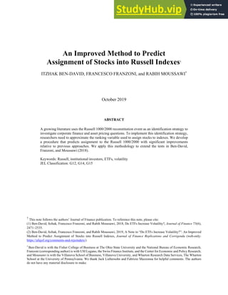
  • 11. 10 are inferior to our rank variable in each of the reconstitution years in our sample. We use the rank variable obtained from our reconstructed market capitalization directly in our regression discontinuity analysis. We investigate further to better understand the reason for the few remaining discrepancies between the Russell index assignments and those based on our rank variable. We notice that in a few cases, Russell considers each class of stock separately, mainly when Russell believes that the common stock share classes act independently of one another. In these cases, Russell differs from CRSP in the issue-company aggregation, as Russell uses issue-level market capitalization instead of total company-level market capitalization in determining index membership. For example, in a few instances, stocks assigned to the Russell 2000 have company-level market capitalization suggesting a Russell 1000 assignment but issue-level market capitalization suggesting a Russell 2000 assignment. In a few other cases, primarily related to recent spinoffs, Russell aggregates the market cap of the parent and spun-off entities and ranks both entities as one. These cases do not seem to follow a systematic pattern, so we cannot infer a rule-based systematic approach to account for them. To study the power of this new ranking variable in predicting index assignment, we run regressions based on equation (1). Following the recommendation in Lee and Lemieux (2010), in Figure 1 we start by plotting the treatment probability (that is, the probability of membership in the Russell 2000 after reconstitution) as a function of the ranking variable. The clear discontinuity at zero testifies to the success of our ranking methodology in closely approximating Russell’s assignment approach.12 12 For graphical convenience, the variable 𝑅𝑎𝑛𝑘 , has been centered on the 1,000th position in terms of market capitalization. Hence, 𝑅𝑎𝑛𝑘 , 0 corresponds to stocks predicted to end up in the Russell 2000, and 𝑅𝑎𝑛𝑘 , 0 corresponds to stocks predicted to end up in the Russell 1000.
  • 12. 11 --- Figure 1 goes about here --- We next report results of the regression analyses in Panel A of Table II.13 The dependent variable is an indicator for whether the stock is assigned to the Russell 2000 in the reconstitution event. The main variable of interest, 𝜏, is a dummy variable that indicates whether our market capitalization variable is above 1,000. We report regressions for four different bandwidths (50, 100, 200, and 400) and specifications including polynomials of the first, second, and third degree. The results show that our ranking variable has statistically strong predictive power for the assignment probability in 11 out of the 12 regressions. The only regression with no statistical significance is that with a bandwidth of ±50 and a third-order polynomial (column (3)). The lack of significance in this specification is arguably due to the fact that the degree of the polynomial is too high for the small number of observations. This analysis also allows us to benchmark our approach against those used by other researchers. We note, however, that our analysis is conducted on somewhat different sample periods from those in other papers, and thus coefficients are not fully comparable. Wei and Young (2017) use a bandwidth of 100 with a linear specification (Table 5, column (2) in their paper). They find a coefficient of 0.72. In the same specification, we obtain an estimate of 0.82 (our Table II, Panel A, column (4)). In a specification with a bandwidth of 200 and a third-order polynomial (their column (1)), their coefficient is 0.55, whereas the corresponding coefficient for us is 0.69 (our Table II, Panel A, column (9)). When we apply Wei and Young’s (2017) procedure to our sample period (2000 to 2006), the estimates are not distinguishable from ours. Appel, Gormley, and Keim (2019b; their Table 2) use bandwidths of 50 and 100 with polynomials of the first to 13 The two-stage least squares estimation includes additional first-stage regressions in which the dependent variables are the assignment variable interacted with 𝑅𝑎𝑛𝑘𝑖,𝑡 and its polynomials. We do not report these regressions to save space because they do not add relevant information.
  • 13. 12 third order. In that paper, five out of the six coefficients are statistically significant and negative. In our Table II, Panel A, columns (1) to (6), all coefficients are positive and five out of the six are statistically significant. Appel, Gormley, and Keim (2019b) also use a bandwidth of 250 and find statistically significant coefficients ranging between 0.09 to 0.65. We use a slightly smaller bandwidth of 200, and the coefficients range between 0.69 and 0.91. --- Table II goes about here --- We further compare the performance of our ranking variable to other candidates based on simply using CRSP or Compustat market capitalization. In Table II, Panel B, we estimate equation (1) for different bandwidths with rankings based on CRSP at the issue and company levels, as well as on Compustat at the issue and company levels. The best-performing of these alternative ranking variables seems to be that based on Compustat at the company level, consistent with the evidence in Table I, Panel B on the number of misclassifications. However, the performance of this alternative ranking variable in predicting assignment is still inferior to that of our ranking variable in Panel A of Table II. The other variables perform even worse. For bandwidths of ±50 or ±100, most of the slopes on 𝜏 are either statistically insignificant or significant but negative. For bandwidths of ±200, the coefficients on the first- and second-degree polynomials are positive, but their magnitude is relatively low. For bandwidths of ±400, all of the coefficients are positive, but the magnitudes are always smaller than the magnitude of the corresponding regression in Panel A. Overall, the coefficients in the regressions in Panel A are larger than the coefficients in each of the corresponding regressions (same bandwidth and polynomial order) in Panel B. To summarize, an assessment of the performance of our ranking variable shows that our measure of total market capitalization has at least comparable and often superior performance in predicting the Russell assignment than that of other viable candidates. Therefore, our variable can
  • 14. 13 help improve the significance of future studies that rely on Russell index assignments for identification. III. An Empirical Application of the New Ranking Variable Ben-David, Franzoni, and Moussawi (2018) use the reconstitution of the Russell 1000/2000 indexes to identify exogenous variation in ETF ownership. The idea is that because most ETFs passively track indexes, a mechanical and unanticipated change in index composition triggers exogenous changes in ETF ownership at the stock level. In that paper, we use CRSP market capitalization in May as a control variable, and thus our methodology is not exposed to the criticism that June market capitalization rankings have attracted (Wei and Young (2017), Appel, Gormley, and Keim (2019b), Glossner (2019)). Overall, the procedure closely follows prior literature that also relies on the Russell reconstitution event (e.g., Appel, Gormley, and Keim (2016)). In this paper, we apply the newly created ranking variable to extend the analysis in Ben- David, Franzoni, and Moussawi (2018) within the framework of a fuzzy RDD. Before doing so, we briefly summarize the methodology that we adopt in the 2018 paper. A. The Approach in Ben-David, Franzoni, and Moussawi (2018) In Ben-David, Franzoni, and Moussawi (2018), we carry out a two-stage least squares estimation. The first stage consists of a regression of ETF ownership on an indicator for whether the stock switched index membership in June. For the Russell 1000 sample, the indicator variable flags stocks that switched to the Russell 2000; for the Russell 2000 sample, the dummy captures a switch to the Russell 1000. In regression form, the first stage is given by equation (4) in the original paper. In the second stage, we regress daily volatility (computed using daily returns within the
  • 15. 14 month) on the fitted value of ETF ownership at the beginning of the month from the first stage. This regression is given by equation (5) in the original paper. We apply this approach to two separate samples that include stock-month observations between June 2000 and May 2007, that is, all of the months following the annual reconstitutions between 2000 and 2006. The first sample comprises all stocks that were in the Russell 1000 as of May of each year, that is, prior to index reconstitution. The second sample comprises all stocks that were in the Russell 2000 as of May. The sample composition is constant for all months between June (the first month after index reconstitution) and May of the following year. The idea underlying the tests is to compare the outcome variables (i.e., volatility) for stocks that changed indexes versus stocks that remained in the same index, in a neighborhood of the cutoff for index switching. Following common practice in the literature, we experiment with various bandwidths around the cutoff (i.e., 50, 100, 200, and 400). To address the concern that index switching is not an exogenous event relative to the dependent variable of interest, we draw inspiration from the RDD methodology. In an RDD, assignment to the treatment group is conditionally exogenous when the econometrician can control for polynomials of the assignment variable. Because the actual Russell rankings in May are not available, we use CRSP market capitalization rankings in May as a proxy. Hence, in our specifications, we control for polynomials of the CRSP May market capitalization rankings to make the treatment variable conditionally exogenous. Additionally, one may be concerned that persistence in volatility could hardwire our results. According to this argument, if lagged volatility increases the probability of switching indexes and volatility is persistent, stocks that switch indexes may display higher future volatility. However, this argument cannot explain why we find that stocks that switch from the Russell 2000
  • 16. 15 to the Russell 1000 display lower volatility (see Table V in the original article, columns (6) to (10)). Moreover, this concern should not arise in the first place because we control for lagged volatility in all of our specifications. B. A Fuzzy RDD to Study the Impact of ETFs on Stock Volatility In what follows, we use the newly created ranking variable within a fuzzy RDD to study the impact of ETF ownership on stock volatility. We refer the reader to the original paper for the motivation behind this analysis. We assume that index redefinition affects stock volatility through ETF ownership. Hence, to study the relation of interest, we can just use volatility as a dependent variable in equation (2). However, because we also wish to express the estimates as a relation between volatility and ETF ownership, we proceed with two-stage least squares estimation. The first stage is a reduced form that combines equations (1) and (2). Specifically, we regress ETF ownership on the variable 𝜏 , and polynomials of the ranking variable: 𝐸𝑇𝐹𝑜𝑤𝑛 , 𝛿 𝛿 𝜏 , 𝛿 , 𝑅𝑎𝑛𝑘 , 𝛿 , 𝜏 , 𝑅𝑎𝑛𝑘 , 𝜖 , . (3) In the second stage, we regress daily volatility computed in the year after reconstitution on instrumented ETF ownership in the December after reconstitution and polynomials of the ranking variable: 𝑉𝑜𝑙𝑎𝑡𝑖𝑙𝑖𝑡𝑦 , 𝛾 𝛾 𝐸𝑇𝐹𝑜𝑤𝑛 , 𝛾 , 𝑅𝑎𝑛𝑘 , 𝛾 , 𝜏 , 𝑅𝑎𝑛𝑘 , 𝜔 , , (4)
  • 17. 16 where the coefficient 𝛾 measures the impact of an expected change in ETF ownership due to index reconstitution, measured in standard deviation units, on stock return volatility after reconstitution, also measured in standard deviation units. In this analysis, we use one observation per stock-year and pool Russell 1000 and 2000 stocks together. The sample period coincides with the reconstitutions between 2000 and 2006, before the banding rule was introduced. ETF ownership is measured at the end of December after reconstitution, and volatility is measured from daily returns in the year after reconstitution. Variable definitions and summary statistics are presented in Appendix C. Before conducting the regression analysis, we provide a graphical summary of the data.14 Figure 2, Panel A presents ETF ownership (as of the December after reconstitution). ETF ownership is expected to be significantly higher by about 40 bps for stocks predicted to end up in the Russell 2000, that is, for rankings above zero, than for those predicted to enter the Russell 1000. The mean of ETF ownership in this sample is about 90 bps and the standard deviation is 84 bps. Hence, the increase is economically significant. When we use lagged ETF ownership in March before reconstitution (Figure 2, Panel B), there is no discontinuity around the cutoff. --- Figure 2 goes about here --- In Figure 3, Panels A and B, we repeat the exercise for total institutional ownership net of ETF ownership. Consistent with prior literature (e.g., Wei and Young (2017)), the panels show that there is no positive jump in total institutional ownership net of ETFs in either the current year or the preceding year. Hence, we conclude that the Russell reconstitution generates significant changes in ETF ownership but not in institutional ownership in general. 14 Based on the argument in Gelman and Imbens (2019) that high-order polynomials lead to noisy estimates, in the graphs we plot linear polynomials estimated with a triangular kernel centered on the cutoff.
  • 18. 17 --- Figure 3 goes about here --- Finally, we present volatility and lagged volatility in Figure 4, Panels A and B. Here, volatility is higher to the right of the cutoff, that is, for stocks that are predicted to end up in the Russell 2000. We again find no visible discontinuity in volatility around the cutoff in the year before the reconstitution event. We next examine the relations of interest in a regression framework. Following equations (1) and (2), we regress ETF ownership measured in the December after reconstitution on the instrumented index assignment indicator. Table II, Panel A presents the results of the first-stage regressions (predicting index assignment). We choose bandwidths around the cutoff ranging from 50 to 400 and present specifications with polynomials ranging from the first to the third order. The regressions include time fixed effects to account for trends in ETF ownership, and we cluster standard errors at the stock level. Table III, Panel A presents results for the second stage on the level of ETF ownership in December, which we standardize by dividing by the standard deviation in the regression sample. The estimates show that ETF ownership is significantly higher for the largest stocks in the Russell 2000 relative to the smallest stocks in the Russell 1000, by 52% to 96% (depending on the bandwidth and polynomial degree) of a standard deviation of the dependent variable. Hence, index assignment generates a large change in ETF ownership, consistent with Figure 2, Panel A (in which ETF ownership is not standardized). --- Table III goes about here --- Finally, Panel B of Table III uses the (standardized) change in ETF ownership between March before reconstitution and December after reconstitution as the dependent variable. This specification addresses the concern that there could be pre-determined differences in ETF
  • 19. 18 ownership around the cutoff. (Panel B of Figure 2 already helps rule out this possibility.) We notice that (instrumented) assignment to treatment corresponds to large changes (of about one standard deviation) in ETF ownership after reconstitution. Table IV, Panel A reports the estimates of equation (4). We control for volatility in the prior year to address the above-mentioned concern that volatility could affect the probability of switching indexes. Across specifications, we find that volatility increases significantly with ETF ownership, by 21% to 76% (depending on the bandwidth and polynomial degree) of a standard deviation for a one-standard-deviation change in ETF ownership. Restricting attention to the bandwidths above 50 for comparability, the magnitude of the median estimate is about 31%, which is almost identical to the result presented in our 2018 paper of about 31% of a standard deviation. --- Table IV goes about here --- In Table IV, Panel B, we modify the specifications from Panel A so that the dependent variable is the year-over-year change in daily volatility around the reconstitution date. In this case, we do not include prior-year volatility among the controls. The estimates are consistent with Panel A and show that volatility increases when ETF ownership rises as a consequence of index reconstitution. We next run regressions in which volatility is the dependent variable in equation (2) and report the results in Table IV, Panel C. The estimates are again significant. Across specifications, volatility is about 20% of a standard deviation higher for stocks in the Russell 2000 than for stocks in the Russell 1000. We present the daily volatility as well as a linear fit in Figure 4, Panel A (in which volatility is not standardized). Gelman and Imbens (2019) argue that controlling for global high-order polynomials in regression discontinuity analyses is a flawed approach because of noisy estimates, sensitivity to
  • 20. 19 the degree of the polynomial, and poor coverage of confidence intervals. They recommend instead using estimators based on local linear or quadratic polynomials. Following their advice, in Table IV, Panel D we modify the specifications of Panel C by including local polynomials of the first and second degree. The results are virtually unchanged in terms of both magnitude and significance.15 To conclude, the fuzzy RDD confirms the results in our 2018 article in terms of both significance and magnitude. IV. Conclusion In this paper we provide an improved methodology for approximating the ranking variable used by Russell to assign stocks to the Russell 1000/2000 indexes. The new ranking variable produces a lower number of misclassified companies relative to other reasonable candidates and a better prediction of the assignment probability than prior studies. Using this variable, we extend and corroborate the findings in Ben-David, Franzoni, and Moussawi (2018). We provide the code for constructing this variable in Appendix B of this paper. The data are available to other researchers wishing to apply this identification strategy per request. Initial submission: June 17, 2019; Accepted: September 6, 2019 Editors: Stefan Nagel, Philip Bond, Amit Seru, and Wei Xiong 15 Specifically, to carry out this estimation, we use the Stata-implemented command –rdrobust– (see Calonico et al. (2017)) with a triangular kernel, clustering standard errors by stock. We include lagged volatility and time fixed effects as controls.
  • 21. 20 REFERENCES Appel, Ian, Todd A. Gormley, and Donald B. Keim, 2016, Passive investors, not passive owners, Journal of Financial Economics 121, 111–141. Appel, Ian, Todd A. Gormley, and Donald B. Keim, 2019a, Standing on the shoulders of giants: The effect of passive investors on activism, Review of Financial Studies 32, 2720–2774. Appel, Ian, Todd A. Gormley, and Donald B. Keim, 2019b, Identification using Russell 1000/2000 Index assignments: A discussion of methodologies, Working paper, University of Pennsylvania. Ben‐David, Itzhak, Francesco Franzoni, and Rabih Moussawi, 2018, Do ETFs increase volatility? Journal of Finance 73, 2471–2535. Bird, Andrew, and Stephen A. Karolyi, 2016, Do institutional investors demand public disclosure? Review of Financial Studies 29, 3245–3277. Boone, Audra L., and Joshua T. White, 2015, The effect of institutional ownership on firm transparency and information production, Journal of Financial Economics 117, 508–533. Calonico, Sebastian, Matias D. Cattaneo, Max H. Farrell, and Rocio Titiunik, 2017, rdrobust: Software for regression discontinuity designs, Stata Journal 17, 372–404. Chang, Yen-Cheng, Harrison Hong, and Inessa Liskovich, 2015, Regression discontinuity and the price effects of stock market indexing, Review of Financial Studies 28, 212–246. Crane, Alan D., Sebastien Michenaud, and James Weston, 2016, The effect of institutional ownership on payout policy: Evidence from index thresholds, Review of Financial Studies 29, 1377–1408. Fich, Eliezer M., Jarrad Harford, and Anh L. Tran, 2015, Motivated monitors: The importance of institutional investors‫׳‬ portfolio weights, Journal of Financial Economics 118, 21–48. FTSE Russell, 2019, Construction and Methodology, Russell U.S. Equity Indexes, May, Available at: https://www.ftse.com/products/downloads/Russell-US-indexes.pdf. Gelman, Andrew, and Guido Imbens, 2019, Why high-order polynomials should not be used in regression discontinuity designs, Journal of Business and Economic Statistics 37, 447–456. Glossner, Simon, 2019, The effects of institutional investors on firm outcomes: Empirical pitfalls of quasi-experiments using Russell 1000/2000 Index reconstitutions, Working paper, University of Pennsylvania.
  • 22. 21 Lee, David S., and Thomas Lemieux, 2010, Regression discontinuity designs in economics, Journal of Economic Literature 48, 281–355. Mullins, William, 2014, The governance impact of index funds: Evidence from regression discontinuity, Working paper, Massachusetts Institute of Technology. Roberts, Michael R., and Tony M. Whited, 2013, Endogeneity in empirical corporate finance, Volume 2A of Handbook of the Economics of Finance (Elsevier, Amsterdam, The Netherlands). Schmidt, Cornelius, and Rüdiger Fahlenbrach, 2017, Do exogenous changes in passive institutional ownership affect corporate governance and firm value? Journal of Financial Economics 124, 285–306. Wei, Wei, and Alex Young, 2017, Selection bias or treatment effect? A re-examination of Russell 1000/2000 Index reconstitution, Working paper, University of Oklahoma.
  • 23. 22 Figure 1. Treatment probability. The figure plots the indicator for membership in the Russell 2000 after reconstitution against market capitalization rankings. A rank of 0 corresponds to the 1,000th stock based on market capitalization. Each bin captures the average of 20 ranks over the sample period. The sample ranges between 2000 and 2006. The solid lines are fitted values from first-order polynomials estimated with a triangular kernel centered on the cutoff. 0.00 0.20 0.40 0.60 0.80 1.00 -400 -200 0 200 400 Rank Treatment Probability
  • 24. 23 Figure 2. ETF ownership. The figure plots ETF ownership in December after reconstitution (Panel A) and in March before reconstitution (Panel B) against market capitalization rankings. A rank of 0 corresponds to the 1,000th stock based on market capitalization. Each bin captures the average of 20 ranks over the sample period. The sample ranges between 2000 and 2006. The solid lines are fitted values from first-order polynomials estimated with a triangular kernel centered on the cutoff. 0.60 0.80 1.00 1.20 1.40 -400 -200 0 200 400 Rank Panel A: ETF Ownership after Reconstitution (%) 0.40 0.60 0.80 1.00 -400 -200 0 200 400 Rank Panel B: ETF Ownership before Reconstitution (%)
  • 25. 24 Figure 3. Other institutions’ ownership. The figure plots ownership by institutions other than ETFs in December after reconstitution (Panel A) and in March before reconstitution (Panel B) against market capitalization rankings. A rank of 0 corresponds to the 1,000th stock based on market capitalization. Each bin captures the average of 20 ranks over the sample period. The sample ranges between 2000 and 2006. The solid lines are fitted values from first-order polynomials estimated with a triangular kernel centered on the cutoff. 62.00 64.00 66.00 68.00 70.00 72.00 -400 -200 0 200 400 Rank Panel A: Other Inst. Ownership after Reconstitution (%) 60.00 62.00 64.00 66.00 68.00 70.00 -400 -200 0 200 400 Rank Panel B: Other Inst. Ownership before Reconstitution (%)
  • 26. 25 Figure 4. Volatility. The figure plots daily volatility in the year after reconstitution (Panel A) and before reconstitution (Panel B) against market capitalization rankings. A rank of 0 corresponds to the 1,000th stock based on market capitalization. Each bin captures the average of 20 ranks over the sample period. The sample ranges between 2000 and 2006. The solid lines are fitted values from first-order polynomials estimated with a triangular kernel centered on the cutoff. 2.200 2.400 2.600 2.800 3.000 -400 -200 0 200 400 Rank Panel A: Volatility after Reconstitution (%) 2.400 2.600 2.800 3.000 3.200 -400 -200 0 200 400 Rank Panel B: Volatility before Reconstitution (%)
  • 27. 26 Table I Performance of Different Computational Approaches for the Assignment Variable The table presents statistics on the performance of our new market capitalization ranking variable compared to other measures of market capitalization. Panel A compares the market capitalization generated by the new variable to the market capitalization generated by alternative variables. Panel B reports the number of misclassifications of Russell 3000 stocks into the Russell 1000 and Russell 2000 indexes during the seven reconstitution years between May 2000 and May 2006. On the rank date of each year, we compute four different market cap measures: (1) the CRSP market cap at the issue level (PERMNO), (2) the total market cap for all issues mapped to the same company in CRSP (PERMCO), (3) the total market cap using the Compustat Securities Daily database aggregated at the company level, and (4) the market cap based on the Compustat Quarterly shares outstanding (CSHOQ). Our ranking methodology relies first on (2), then (3) when (1) is missing, and (4) when it is higher than (2) and (3). Ranking is performed according to the ranking of the Russell 3000 using their various market capitalization measures computed at the end of the rank date. The number of Russell 3000 stocks on the reconstitution date at the end of June is sometimes less than 3,000 because Russell follows a “no-replacement” rule. Panel A: Deviation between Our Market Capitalization Variable and Other Proxies of Market Capitalization Deviation between the new market cap measure and existing variables CRSP Issue Market Cap CRSP Issuer Total Market Cap Compustat Securities Total Market Cap Compustat Quarterly Shares Oustanding (CSHOQ) <-10% 0.0% 0.0% 0.1% 0.0% -10% to -1% 0.0% 0.0% 0.1% 0.0% -1% to 0.1% 0.0% 0.0% 0.1% 0.0% -0.1% to 0.1% 78.4% 80.0% 75.5% 95.2% 0.1% to 1% 9.4% 9.6% 12.3% 2.7% 1% to 10% 4.9% 4.9% 6.2% 1.1% >10% 7.3% 5.5% 5.5% 0.6% Other market capitalization variables
  • 28. 27 Table I Performance of Different Computational Approaches for the Assignment Variable (Cont.) Panel B: Misclassification Errors in the Russell Indexes by the Different Computational Approaches Russell 3000 Russell 1000 Russell 2000 Russell 1000 Russell 2000 Russell 1000 Russell 2000 Russell 1000 Russell 2000 Russell 1000 Russell 2000 Russell 1000 Russell 2000 31-May-2000 3000 1000 2000 8 8 29 30 26 27 26 30 5 12 31-May-2001 3000 1000 2000 5 5 31 31 28 28 24 35 2 13 31-May-2002 3000 1000 2000 4 4 26 26 21 21 21 29 5 16 31-May-2003 3000 1000 2000 2 2 22 22 19 19 18 24 3 15 31-May-2004 2998 999 1999 3 4 21 22 17 18 18 27 3 16 31-May-2005 3000 1000 2000 4 4 18 19 18 19 14 21 2 15 31-May-2006 2987 994 1993 1 7 18 24 17 23 14 24 1 17 Misclassification errors 27 34 165 174 146 155 135 190 21 104 Total number of misclassified securities # Misclassification errors Using CRSP Issuer Total Market Cap Using Compustat Securities Total Market Cap Using Compustat Quarterly Shares Oustanding 61 339 301 325 125 Using CRSP Issue Market Cap Reconstitution rank date Our methodology # Stocks
  • 29. 28 Table II First Stage: Predicting Index Membership The table reports estimates of equation (1). The sample includes one stock observation per year. The dependent variable is index assignment. Time fixed effects are included in all specifications. We report estimates from different bandwidths around the cutoff for reconstitution (50, 100, 200, and 400 ranks) and specifications with different polynomials of the ranking variable (from the first to the third degree). Standard errors are clustered by stock. The sample spans the Russell reconstitutions between 2000 and 2006. Panel A: First Stage Using the New Variable Dependent variable: Bandwidth: (1) (2) (3) (4) (5) (6) (7) (8) (9) (10) (11) (12)  0.684*** 0.415*** 0.173 0.824*** 0.656*** 0.468*** 0.906*** 0.806*** 0.688*** 0.947*** 0.897*** 0.827*** (12.598) (4.227) (1.195) (27.301) (11.212) (5.215) (55.765) (24.303) (12.929) (111.103) (49.964) (27.771) Rank 0.005*** 0.019*** 0.045*** 0.001*** 0.006*** 0.017*** 0.000*** 0.002*** 0.006*** 0.000*** 0.001*** 0.002*** (4.325) (3.739) (3.194) (4.309) (4.120) (3.912) (4.182) (4.301) (4.272) (4.213) (4.041) (4.343) Rank ×  -0.001 0.002 0.005 -0.000 -0.000 0.000 -0.000 -0.000 -0.001 -0.000 -0.000 -0.000 (-0.369) (0.276) (0.255) (-0.406) (-0.104) (0.077) (-0.520) (-0.307) (-0.283) (-0.058) (-0.325) (-0.464) Rank2 0.000*** 0.002*** 0.000*** 0.000*** 0.000*** 0.000*** 0.000*** 0.000*** (3.431) (2.857) (3.981) (3.704) (4.268) (4.181) (3.971) (4.349) Rank2 ×  -0.001*** -0.003*** -0.000*** -0.001*** -0.000*** -0.000*** -0.000*** -0.000*** (-5.243) (-4.527) (-5.476) (-5.381) (-5.559) (-5.441) (-5.112) (-5.531) Rank3 0.000*** 0.000*** 0.000*** 0.000*** (2.691) (3.580) (4.120) (4.357) Rank3 ×  0.000 0.000 -0.000 -0.000 (0.244) (0.189) (-0.256) (-0.495) Time F.E. yes yes yes yes yes yes yes yes yes yes yes yes Observations 673 673 673 1,354 1,354 1,354 2,699 2,699 2,699 5,391 5,391 5,391 R2 0.831 0.844 0.850 0.905 0.910 0.915 0.945 0.947 0.948 0.970 0.970 0.971 R2000 ± 50 ± 100 ± 200 ± 400
  • 30. 29 Table II First Stage: Predicting Index Membership (Cont.) Panel B: First Stage Using the Other Proxies of Market Capitalization Dependent variable: Bandwidth: Polynomial order: 1st 2nd 3rd 1st 2nd 3rd 1st 2nd 3rd 1st 2nd 3rd (1) (2) (3) (4) (5) (6) (7) (8) (9) (10) (11) (12) τ -0.152*** -0.109 0.082 0.171*** -0.206*** -0.222*** 0.506*** 0.129*** -0.161*** 0.702*** 0.467*** 0.204*** (-3.263) (-1.501) (0.834) (4.902) (-4.312) (-3.288) (18.940) (3.581) (-3.582) (38.828) (16.838) (5.852) Observations 682 682 682 1,351 1,351 1,351 2,698 2,698 2,698 5,383 5,383 5,383 R2 0.557 0.561 0.583 0.703 0.760 0.760 0.751 0.807 0.830 0.831 0.855 0.875 τ -0.135*** -0.377*** -0.078 0.284*** -0.186*** -0.388*** 0.583*** 0.229*** -0.096** 0.749*** 0.549*** 0.300*** (-3.160) (-5.631) (-0.857) (7.951) (-4.219) (-6.131) (21.870) (6.248) (-2.266) (43.232) (19.647) (8.446) Observations 679 679 679 1,355 1,355 1,355 2,706 2,706 2,706 5,394 5,394 5,394 R2 0.690 0.705 0.730 0.726 0.804 0.813 0.778 0.825 0.854 0.852 0.869 0.886 τ -0.177*** -0.284*** 0.070 0.225*** -0.227*** -0.358*** 0.551*** 0.173*** -0.153*** 0.735*** 0.514*** 0.249*** (-4.174) (-4.180) (0.754) (6.787) (-5.278) (-5.316) (21.393) (5.128) (-3.800) (43.790) (19.224) (7.528) Observations 682 682 682 1,353 1,353 1,353 2,700 2,700 2,700 5,387 5,387 5,387 R2 0.684 0.687 0.731 0.739 0.816 0.819 0.780 0.835 0.865 0.853 0.874 0.893 τ 0.463*** 0.083 -0.203** 0.700*** 0.425*** 0.143** 0.840*** 0.674*** 0.475*** 0.915*** 0.823*** 0.705*** (8.885) (1.133) (-2.194) (20.782) (7.798) (2.057) (43.388) (18.663) (9.324) (86.896) (38.856) (21.368) Observations 676 676 676 1,354 1,354 1,354 2,701 2,701 2,701 5,385 5,385 5,385 R2 0.794 0.842 0.857 0.868 0.895 0.913 0.921 0.931 0.940 0.956 0.959 0.963 Rank based on CRSP issue level Rank based on CRSP company level Rank based on Compustat issue level Rank based on Compustat company level R2000 ± 50 ± 100 ± 200 ± 400
  • 31. 30 Table III Second Stage: ETF Ownership The table reports estimates of equation (2). The sample includes one stock observation per year. In Panel A, the dependent variable is ETF ownership in December after the Russell index reconstitution, expressed in standard deviation units. In Panel B, the dependent variable is the March-to-December change in ETF ownership expressed in standard deviation units. Time fixed effects are included in all specifications. We report estimates from different bandwidths around the cutoff for reconstitution (50, 100, 200, and 400 ranks) and specifications with different polynomials of the ranking variable (from the first to the third degree). Standard errors are clustered by stock. The sample spans the Russell reconstitutions between 2000 and 2006. Panel A: ETF Ownership Dependent variable: Bandwidth: (1) (2) (3) (4) (5) (6) (7) (8) (9) (10) (11) (12) IV(R2000) 0.535*** 0.964** 2.142 0.550*** 0.524*** 0.813*** 0.551*** 0.587*** 0.613*** 0.561*** 0.523*** 0.598*** (3.888) (2.577) (1.443) (6.478) (3.459) (2.680) (9.907) (6.183) (4.261) (13.557) (8.673) (6.911) Rank 0.001 -0.018 -0.038 -0.001 -0.002 0.001 -0.002*** -0.003** 0.002 -0.000 -0.002*** -0.004*** (0.492) (-1.559) (-0.710) (-0.906) (-0.490) (0.081) (-4.153) (-2.160) (0.423) (-1.251) (-3.834) (-2.720) Rank2 0.001 0.006 -0.000 0.001 0.000 0.000 -0.000 0.000 (1.366) (1.138) (-0.226) (1.199) (0.502) (0.327) (-0.787) (1.129) Rank3 -0.000 0.000 0.000 -0.000 (-0.157) (0.312) (1.299) (-1.077) IV(R2000) × Rank -0.001 -0.009 -0.071 0.000 0.002 -0.012 0.001*** 0.001 -0.002 0.000* 0.002*** 0.001 (-0.308) (-0.598) (-0.784) (0.447) (0.418) (-1.031) (3.307) (1.020) (-0.539) (1.721) (3.524) (1.133) IV(R2000) × Rank2 -0.000 -0.002 0.000 -0.000 0.000 -0.000 0.000*** 0.000 (-0.448) (-0.737) (0.339) (-1.190) (0.275) (-0.982) (3.120) (0.233) IV(R2000) × Rank3 -0.000 -0.000 -0.000 -0.000 (-0.736) (-1.249) (-1.080) (-0.284) Time F.E. yes yes yes yes yes yes yes yes yes yes yes yes Observations 673 673 673 1,354 1,354 1,354 2,699 2,699 2,699 5,391 5,391 5,391 ETF ownership in December (standardized) ± 50 ± 200 ± 400 ± 100
  • 32. 31 Table III Second Stage: ETF Ownership (Cont.) Panel B: Change in ETF Ownership Dependent variable: Bandwidth: (1) (2) (3) (4) (5) (6) (7) (8) (9) (10) (11) (12) IV(R2000) 0.905*** 0.924** 2.029 1.151*** 0.900*** 1.043** 1.228*** 1.280*** 1.188*** 1.213*** 1.399*** 1.393*** (4.645) (2.051) (1.411) (9.435) (3.994) (2.466) (14.903) (8.849) (5.621) (20.326) (14.234) (9.569) Rank -0.001 -0.011 -0.043 -0.001 -0.007 -0.007 0.000 -0.003 -0.008 0.001*** -0.001 -0.000 (-0.322) (-0.759) (-0.723) (-0.542) (-1.137) (-0.530) (0.848) (-1.352) (-1.182) (2.586) (-0.901) (-0.138) Rank2 0.000 0.005 -0.000 0.000 0.000 -0.000 0.000*** 0.000 (0.038) (0.955) (-1.601) (0.263) (0.542) (-0.592) (2.818) (0.372) Rank3 -0.000 -0.000 -0.000 0.000 (-0.347) (-0.011) (-0.817) (0.248) IV(R2000) × Rank 0.002 0.006 -0.045 -0.001 0.008 0.002 -0.002*** -0.001 0.004 -0.001*** -0.002*** -0.002 (0.419) (0.301) (-0.507) (-0.906) (1.390) (0.129) (-4.109) (-0.372) (0.678) (-7.792) (-2.680) (-1.084) IV(R2000) × Rank2 0.000 -0.002 0.000* -0.000 0.000 0.000 -0.000 -0.000 (0.267) (-0.509) (1.769) (-0.124) (0.626) (1.045) (-0.909) (-0.238) IV(R2000) × Rank3 -0.000 -0.000 0.000 -0.000 (-0.525) (-0.399) (1.008) (-0.096) Time F.E. yes yes yes yes yes yes yes yes yes yes yes yes Observations 669 669 669 1,346 1,346 1,346 2,682 2,682 2,682 5,364 5,364 5,364 March-to-December Change in ETF ownership (standardized) ± 50 ± 200 ± 400 ± 100
  • 33. 32 Table IV Volatility The table reports estimates of equations (2) and (4). The sample includes one stock observation per year. Panel A follows equation (4), and the dependent variable is daily volatility computed in the year after the Russell index reconstitution and expressed in standard deviation units. Panel B also follows equation (4), and the dependent variable is the year-over-year change in daily volatility around the reconstitution. Panel C follows equation (2), and the dependent variable is daily volatility in the year after reconstitution. In Panels A, B, and C, the polynomials are global. In Panel D, we implement the fuzzy RDD using local polynomials. For this estimation, we use first- and second-degree local polynomials with a triangular kernel. All of the specifications include time fixed effects. We report estimates from different bandwidths around the cutoff for reconstitution (50, 100, 200, and 400 ranks) and specifications with different polynomials of the ranking variable (from the first to the third degree). Standard errors are clustered by stock. The sample spans the Russell reconstitutions between 2000 and 2006. Panel A: Volatility on ETF Ownership Dependent variable: Bandwidth: (1) (2) (3) (4) (5) (6) (7) (8) (9) (10) (11) (12) IV(ETF ownership) 0.760*** 0.573* 0.344 0.412*** 0.714** 0.719* 0.305*** 0.295** 0.586*** 0.206*** 0.300*** 0.313*** (2.692) (1.775) (1.060) (3.103) (2.299) (1.900) (3.742) (2.341) (2.659) (3.992) (3.333) (2.732) Rank -0.004 -0.007 0.019 -0.001 -0.004 -0.007 -0.001*** -0.000 -0.004 -0.000* -0.001** -0.001 (-1.442) (-0.770) (0.977) (-1.496) (-0.947) (-0.798) (-2.825) (-0.041) (-1.206) (-1.924) (-2.111) (-1.224) Rank2 -0.000 0.001 -0.000 -0.000 0.000 -0.000 -0.000* -0.000 (-0.434) (1.247) (-0.662) (-0.471) (0.754) (-1.020) (-1.794) (-0.646) Rank3 0.000 -0.000 -0.000 -0.000 (1.281) (-0.325) (-1.090) (-0.301) Rank ×  -0.002 0.013 -0.019 0.000 -0.002 0.003 0.001** -0.001 -0.002 0.000 0.001 0.001 (-0.634) (1.102) (-0.677) (0.032) (-0.445) (0.204) (2.202) (-0.509) (-0.429) (0.015) (1.471) (0.876) Rank2 ×  -0.000 -0.001 0.000 0.000 -0.000 0.000* 0.000 0.000 (-0.758) (-0.993) (1.261) (0.303) (-0.093) (1.860) (1.314) (0.409) Rank3 ×  -0.000 0.000 -0.000 0.000 (-1.035) (0.391) (-0.523) (0.267) lag(Volatility) 0.898*** 0.881*** 0.860*** 0.857*** 0.883*** 0.883*** 0.829*** 0.828*** 0.853*** 0.822*** 0.830*** 0.831*** (21.301) (21.295) (21.823) (31.325) (23.434) (21.491) (43.570) (40.018) (31.050) (65.074) (57.989) (53.473) Time F.E. yes yes yes yes yes yes yes yes yes yes yes yes Observations 673 673 673 1,354 1,354 1,354 2,699 2,699 2,699 5,391 5,391 5,391 ± 50 ± 200 ± 400 Daily stock volatility (standardized) ± 100
  • 34. 33 Table IV Volatility (Cont.) Panel B: Change in Volatility Dependent variable: Bandwidth: (1) (2) (3) (4) (5) (6) (7) (8) (9) (10) (11) (12) IV(ETF ownership) 1.443*** 1.052* 0.590 0.732*** 1.348** 1.344** 0.555*** 0.526** 1.042*** 0.397*** 0.560*** 0.711*** (2.857) (1.760) (0.942) (3.121) (2.473) (2.009) (3.982) (2.409) (2.732) (3.743) (3.203) (2.927) Rank -0.008 -0.012 0.039 -0.002* -0.010 -0.013 -0.002*** -0.001 -0.008 -0.001** -0.002** -0.005* (-1.563) (-0.690) (1.046) (-1.698) (-1.185) (-0.880) (-3.399) (-0.238) (-1.437) (-2.393) (-2.187) (-1.646) Rank2 -0.000 0.002 -0.000 -0.000 0.000 -0.000 -0.000* -0.000 (-0.316) (1.320) (-0.872) (-0.473) (0.666) (-1.216) (-1.751) (-1.066) Rank3 0.000 -0.000 -0.000 -0.000 (1.342) (-0.283) (-1.279) (-0.750) Rank ×  -0.004 0.024 -0.037 0.000 -0.003 0.005 0.001** -0.001 -0.001 0.000 0.002 0.003 (-0.587) (1.071) (-0.703) (0.239) (-0.283) (0.240) (2.241) (-0.300) (-0.179) (0.183) (1.568) (0.948) Rank2 ×  -0.000 -0.002 0.000 0.000 -0.000 0.000* 0.000 0.000 (-0.880) (-1.101) (1.474) (0.314) (-0.163) (1.925) (1.192) (1.084) Rank3 ×  -0.000 0.000 -0.000 0.000 (-1.055) (0.365) (-0.339) (0.204) Time F.E. yes yes yes yes yes yes yes yes yes yes yes yes Observations 673 673 673 1,354 1,354 1,354 2,699 2,699 2,699 4,048 4,048 4,048 ± 100 Daily stock volatility (year-over-year change, standardized) ± 50 ± 200 ± 400
  • 35. 34 Table IV Volatility (Cont.) Panel C: Volatility on Index Assignment Dependent variable: Bandwidth: (1) (2) (3) (4) (5) (6) (7) (8) (9) (10) (11) (12) R2000 0.379*** 0.492 0.319 0.226*** 0.361*** 0.488** 0.161*** 0.188*** 0.346*** 0.115*** 0.157*** 0.176*** (3.696) (1.640) (0.414) (3.449) (3.073) (2.100) (3.841) (2.678) (3.173) (4.044) (3.555) (2.816) Rank -0.002 -0.001 -0.063 -0.001 -0.005 0.001 0.000 -0.002 -0.001 -0.000 -0.000 -0.001 (-0.756) (-0.102) (-1.556) (-0.700) (-1.386) (0.073) (0.457) (-1.592) (-0.174) (-0.450) (-0.112) (-0.487) Rank2 0.000 -0.000 0.000 0.000 0.000 0.000* 0.000 0.000 (0.465) (-0.074) (1.497) (0.925) (0.474) (1.954) (1.194) (0.626) Rank3 -0.000 0.000 0.000 -0.000 (-1.445) (0.657) (0.482) (-0.471) Rank ×  -0.004* -0.009 0.032 -0.001 -0.002 -0.011 -0.000* 0.000 -0.004 -0.000 -0.000 -0.000 (-1.822) (-0.769) (0.636) (-1.266) (-0.765) (-1.123) (-1.953) (0.266) (-1.615) (-1.590) (-1.293) (-0.508) Rank2 ×  -0.000 0.002 -0.000 -0.000 0.000 -0.000 -0.000 -0.000 (-0.499) (0.948) (-0.403) (-1.036) (0.741) (-1.627) (-0.934) (-0.159) Rank3 ×  0.000 -0.000 -0.000* -0.000 (1.089) (-1.029) (-1.693) (-0.009) lag(Volatility) 0.816*** 0.813*** 0.839*** 0.818*** 0.818*** 0.813*** 0.801*** 0.800*** 0.801*** 0.802*** 0.802*** 0.802*** (29.199) (27.814) (16.675) (36.285) (36.206) (34.527) (48.586) (48.486) (48.861) (67.799) (67.836) (67.802) Time F.E. yes yes yes yes yes yes yes yes yes yes yes yes Observations 697 697 697 1,396 1,396 1,396 2,794 2,794 2,794 5,591 5,591 5,591 ± 100 Daily stock volatility (standardized) ± 50 ± 200 ± 400
  • 36. 35 Table IV Volatility (Cont.) Panel D: Volatility on Index Assignment, Local Polynomials Dependent variable: Bandwidth: ± 50 ± 100 ± 200 ± 400 ± 50 ± 100 ± 200 ± 400 (1) (2) (3) (4) (5) (6) (7) (8) R2000 0.404*** 0.274*** 0.172*** 0.132*** 0.434 0.409*** 0.253*** 0.165*** (0.136) (0.075) (0.047) (0.031) (0.403) (0.145) (0.078) (0.048) Order Loc. Poly. 1 1 1 1 2 2 2 2 Kernel Type Triangular Triangular Triangular Triangular Triangular Triangular Triangular Triangular lag(Volatility) yes yes yes yes yes yes yes yes Time F.E. yes yes yes yes yes yes yes yes Observations 697 1,396 2,794 5,591 697 1,396 2,794 5,591 Daily stock volatility (standardized)
  • 37. 36 Appendix A: Historical Russell Rank Dates and Reconstitution Dates We are grateful to FTSE Russell for providing a detailed calendar of its historical index reconstitutions. According to Russell, US indexes were rebalanced quarterly between 1979 to 1986, semi-annually from 1987 to 1989, and annually after June 1989. For time periods prior to when reconstitution was performed annually, security lists were ranked based on the month of rebalancing. For example, for March 1979, the securities were ranked based on their total market capitalization on March 31, 1979. When the reconstitution was first performed annually in June 1989, the reconstitution date was the final business day of June. In 2004, Russell revised the reconstitution date to the last Friday in June. In 2007, the reconstitution was effective after the close on the last Friday in June unless the last Friday occurred on the 28th, 29th, or 30th (if so, reconstitution occurred on the prior Friday). In 2013, the reconstitution date rule was changed to after the close on the last Friday in June unless the last Friday occurs on the 29th or 30th. If so, reconstitution will occur the prior Friday. Reconstitution Date Rank Date Preliminary Announcement Date Reconstitution Date Rank Date Preliminary Announcement Date June 28, 2019 May 10, 2019 June 7, 2019 June 28, 2002 May 31, 2002 June 14, 2002 June 22, 2018 May 11, 2018 June 8, 2018 June 29, 2001 May 31, 2001 June 8, 2001 June 23, 2017 May 12, 2017 June 9, 2017 June 30, 2000 May 31, 2000 June 9, 2000 June 24, 2016 May 27, 2016 June 10, 2016 June 30, 1999 May 28, 1999 June 11, 1999 June 26, 2015 May 29, 2015 June 12, 2015 June 30, 1998 May 29, 1998 June 12, 1998 June 27, 2014 May 30, 2014 June 13, 2014 June 30, 1997 May 30, 1997 June 13, 1997 June 28, 2013 May 31, 2013 June 14, 2013 June 28, 1996 May 31, 1996 June 14, 1996 June 22, 2012 May 31, 2012 June 8, 2012 June 30, 1995 May 31, 1995 June 24, 2011 May 31, 2011 June 10, 2011 June 30, 1994 May 31, 1994 June 25, 2010 May 28, 2010 June 11, 2010 June 30, 1993 May 28, 1993 June 26, 2009 May 29, 2009 June 12, 2009 June 30, 1992 May 29, 1992 June 27, 2008 May 30, 2008 June 13, 2008 June 28, 1991 May 31, 1991 June 22, 2007 May 31, 2007 June 11, 2007 June 29, 1990 May 31, 1990 June 30, 2006 May 31, 2006 June 16, 2006 June 30, 1989 May 31, 1989 June 24, 2005 May 31, 2005 June 10, 2005 June 25, 2004 May 28, 2004 June 11, 2004 June 30, 2003 May 30, 2003 June 13, 2003
  • 38. 37 Appendix B: Code Logic to Generate the Russell Rank Proxy The Russell 3000 constituent data between 2000 and 2006 are not available on Wharton Research Data Services (WRDS) as of the publication of this article, but we make it available to researchers who ask. We matched each Russell constituent to its CRSP PERMNO and Compustat’s GVKEY using historical CUSIP information in CRSP MSENAMES and Compustat Snapshot’s CNSECURITY datasets. The resulting dataset, Russell_1, is then merged with the CRSP, Compustat Securities, and Compustat Quarterly information to compute the RANK variable, which represents our proxy for the Russell true rank. CRSP and COMP libraries are the SAS libraries for CRSP and Compustat datasets on WRDS, and %POPULATE is the SAS macro in the WRDS Research Macro section. /* Create Market Capitalization Variables using CRSP Daily Stock Data */ proc sql; create table mktcap_crsp as select distinct date, permno, permco, abs(prc*shrout)/1000 as mktcap_CRSP format dollar12.3, sum(abs(prc*shrout)/1000) as tot_mktcap_CRSP format dollar12.3 from crsp.dsf where month(date) in (5,6) and date>="15MAY2000"d and date<="30JUN2008"d group by date, permco; quit; /* Create Market Capitalization Variable using Compustat Securities Daily */ /* Compustat has preferred stocks, warrants, rights, etc. */ /* Only keep US listed common/ordinary issues */ proc sql; create table mktcap_comp (rename=datadate=date) as select distinct gvkey, datadate, sum(prccd*cshoc/1000000) as tot_mktcap_COMP format dollar12.3 from compna.secd where datadate>='01JAN1999'd and month(datadate) in (5,6) and curcdd='USD' and tpci in ('0') group by gvkey, datadate; quit; /* Extract the total shares outstanding reported in the 10-Qs and 10-Ks */ data cshoq; set compna.fundq; where not missing(cshoq); * could lag datadate by two months, but not necessary; * datadate=intnx("month",datadate,2,"e"); keep gvkey datadate cshoq fyr; run; /* Add the adjustment factor as of fiscal quarter end */ proc sql; create table cshoq as select a.*, b.iid, b.ajexm as ajexq from cshoq as a left join compna.secm as b on a.gvkey=b.gvkey and intnx("month",a.datadate,0,"e")=intnx("month",b.datadate,0,"e"); quit; proc sql;
  • 39. 38 create table cshoq as select distinct gvkey, iid, datadate, cshoq, ajexq from cshoq group by gvkey, iid, datadate having cshoq=max(cshoq); quit; /* populate the data forward on a monthly frequency */ %POPULATE (INSET=cshoq,OUTSET=cshoq,DATEVAR=datadate,IDVAR=gvkey iid, FORWARD_MAX=12); /* Compute total market capitalization including non-traded share classes */ /* Merge with Compustat Securities data for traded share classes market cap */ data secm; set compna.secm; * keep only US listed common/ordinary issues; where curcdm='USD' and datadate>='01JAN1999'd and tpci in ('0'); cshom=cshom/1000000; mktcap_COMP=cshom*prccm; run; proc sql; create table secm as select distinct gvkey, iid, intnx("month",datadate,0,"e") as date format date9., datadate, ajexm, sum(cshom) as tot_cshom, sum(mktcap_COMP) as tot_mktcap_COMP, sum(mktcap_COMP*prccm)/sum(mktcap_COMP*(abs(prccm)>0)) as prccm_vw /* mktcap-weighted average price per share class */ from secm group by gvkey, datadate; quit; data secm; merge secm(in=a) cshoq (rename=(mdate=date)); by gvkey iid date; if a; run; proc sort data=secm nodupkey; by gvkey iid date; run; data secm; set secm; by gvkey iid date; if missing(ajexm) then ajexm=1; if missing(ajexq) then ajexq=ajexm; /* tot_mktcap_COMP is total market cap of all traded share classes */ /* Shares of non-tradable share classes = cshoq*ajexq-tot_cshom*ajexm */ tot_mktcap_COMP_ALL=(cshoq*ajexq-tot_cshom*ajexm)*prccm_vw/ajexm + tot_mktcap_COMP; if cshoq*ajexq-tot_cshom*ajexm<0 then tot_mktcap_COMP_ALL=tot_mktcap_COMP; format tot_cshom csho: comma12.3 tot_mktcap_comp tot_mktcap_COMP_ALL dollar12.3; run; proc sql; create table secm
  • 40. 39 as select distinct gvkey, date, mean(tot_mktcap_COMP_ALL) as tot_mktcap_COMP_ALL format dollar12.3 from secm group by gvkey, date order by gvkey, date; quit; /* check */ proc sort data=secm nodupkey; by gvkey date; run; /* Add CRSP Market Cap data on the closest trading day */ proc sql; create table Russell_2 as select a.*, b.date as date_crsp, b.mktcap_CRSP, b.tot_mktcap_CRSP from Russell_1 as a left join mktcap_crsp as b on int(a.permno)=b.permno and a.tdate-15<=b.date group by a.cusip, a.date, a.permno having abs(a.tdate-b.date)=min(abs(a.tdate-b.date)); quit; /* Add Compustat Market Cap data on the closest trading day */ proc sql; create table Russell_3 as select a.*, b.date as date_comp, b.tot_mktcap_COMP from Russell_2 as a left join mktcap_comp as b on a.gvkey=b.gvkey and a.tdate-15<=b.date group by a.cusip, a.date, a.permno having abs(a.tdate-b.date)=min(abs(a.tdate-b.date)); quit; /* Add Compustat Market Cap data of ALL shares outstanding */ proc sql; create table Russell_4 as select distinct a.*, tot_mktcap_COMP_ALL from Russell_3 as a left join secm as b on a.gvkey=b.gvkey and a.date=b.date; quit; /* Create the Ranks: Compute the Russell’s Total Market Cap Proxy */ data Russell_5; set Russell_4; /* 1. Use CRSP market cap */ tot_mktcap_r3=tot_mktcap_CRSP; /* 2. if missing, use Compustat market cap */ if missing(tot_mktcap_r3) then tot_mktcap_r3=tot_mktcap_COMP; /* 3. Use Compustat total market cap if Compustat total market cap is higher due to OTC shares or non-tradable shares */ if missing(tot_mktcap_r3) then tot_mktcap_r3=tot_mktcap_COMP_ALL; if tot_mktcap_COMP_ALL>tot_mktcap_r3 then tot_mktcap_r3=tot_mktcap_COMP_ALL; format mkt_value tot_mktcap_r3 dollar12.3; run; proc rank data= Russell_5 out= Russell_6 descending; by date; where mkt_value>0; var tot_mktcap_r3; ranks Rank; run;
  • 41. 40 Appendix C: Variable Definitions and Summary Statistics The table presents summary statistics for the variables used in the regressions presented in Tables 3 and 4. Note that the regressions in these tables are presented using standardized variables. All variables are winsorized at the 1% and 99% levels. Panel A: Variable Definitions Institutional ownership in December: Institutional ownership is computed using the Thomson- Reuters 13F Institutional Ownership database. For each stock, we sum the ownership by all institutions in December and scale that number by the total shares outstanding of the stock. ETF ownership in December: ETF ownership is computed using the Thomson-Reuters Global Ownership database. We first identify all ETFs using the fund CUSIP and ticker information in the OWNSECMAP and OWNFUNDTIC datasets, and then merge it with the list of ETF CUSIP and tickers extracted from CRSP, Compustat, and the OWNSECINFO dataset (using the SecClsCode = “ETF” condition). In December, we use the nearest fund holding reports and sum the ownership by all ETFs in each stock and then scale that number by the total shares outstanding of that stock. Daily stock volatility: Using the CRSP daily stock file data, we compute the stock volatility measure as the standard deviation of the log (1+ daily returns) for all daily observations between the reconstitution effective date (July 1) and the next reconstitution effective date (June 30 of the following year). Panel B: Summary Statistics Variable N Mean Std Dev Min Median Max Institutional ownership in December 20,457 0.6097 0.2517 0.065 0.6402 1.1049 ETF ownership in December 20,037 0.0093 0.0084 0.0001 0.007 0.0377 Daily stock volatility 20,945 0.0289 0.0179 0.0082 0.0237 0.1012