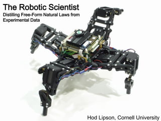
Distilling Free-Form Natural Laws from Experimental Data
•
1 j'aime•3,629 vues

The document describes research on using symbolic regression to infer mathematical models from experimental data. Symbolic regression evolves computer programs that best fit the data, such as equations composed of basic arithmetic operations and functions. The approach is able to recover known models of various physical systems from sample data alone. It can also infer novel models of biological networks and other complex systems directly from experimental measurements. The ability to distill natural laws from data has applications in scientific discovery, engineering design, and other fields.

Recommandé
Contenu connexe
Tendances
Tendances (19)
Similaire à Distilling Free-Form Natural Laws from Experimental Data
Similaire à Distilling Free-Form Natural Laws from Experimental Data (20)
Plus de swissnex San Francisco
Plus de swissnex San Francisco (20)
Dernier
Dernier (20)
Distilling Free-Form Natural Laws from Experimental Data
- 1. The Robotic Scientist Distilling Free-Form Natural Laws from Experimental Data Hod Lipson, Cornell University
- 3. Lipson & Pollack, Nature 406, 2000
- 8. Camera Camera View
- 10. Adapting in simulation Simulator Evolve Controller Crossing The In Simulation Reality Gap Download Try it in reality!
- 11. Adapting in reality Evolve Controller In Reality Too many Physical Trials Try it !
- 12. Simulation & Reality “Simulator” Evolve Simulator Evolve Controller Evolve Simulators Evolve Robots Build Collect Sensor Data Try it in reality!
- 13. Tilt Sensors Servo Actuators
- 16. Emergent Self-Model With Josh Bongard and Victor Zykov, Science 2006
- 17. Damage Recovery With Josh Bongard and Victor Zykov, Science 2006
- 20. System Identification ?
- 21. Perturbations
- 22. Photo: Floris van Breugel
- 23. Structural Damage Diagnosis With Wilkins Aquino
- 24. Symbolic Regression What function describes this data? f(x)=exsin(|x|) John Koza, 1992
- 25. Encoding Equations Building Blocks: + - * / sin cos exp log … etc f(x) sin(x2) * x1*sin(x2) – sin (x1 – 3)*sin(x2) (x1 – 3)*sin(-7 + x2) x1 3 + x2 -7 John Koza, 1992
- 26. + × sin 1.2 – x x 2 Models: Expression trees Experiments: Data-points Subject to mutation and selection Subject to mutation and selection {const,+,-,*,/,sin,cos,exp,log,abs} Michael D. Schmidt, Hod Lipson (2006)
- 27. Solution Accuracy Coevolved Dataset Entire Dataset
- 28. Solution Complexity 35 33 Entire Dataset 31 Solution Size (# of nodes) 29 27 25 23 21 19 Coevolved Dataset Coevolution Exact 17 15 0 5000 10000 15000 Generations
- 30. Semi-empirical mass formula Modeling the binding energy of an atomic nucleus Inferred Formula: 0.39Z 2 17.29( N Z ) 2 EB 14.83 13.43 A 12.39 A 0 .64 0.26 R2 = 0.99944 A A Weizsäcker’s Formula: Z Z 1 A 2Z 2 A, Z E a Aa A a B V 23 S a C 13 A R2 = 0.999915 A A 0 Z , N even A, Z 0 A odd 0 aP A1 2 0 Z , N odd
- 32. Systems of Differential Equations • Regress on derivative State Variables Derivatives time x1 x2 … dx1/dt x2/dt … 0 3.4 -1.7 … -2.0 8.0 … 0.1 3.2 -0.9 … -1.0 8.0 … 0.2 3.1 -0.1 … -4.0 1.3 … 0.3 2.7 1.2 … -5.7 1.9 … … … … … … … …
- 33. Inferring Biological Networks dS1 S1 * A3 dS1 2.5 100 S1 * A3 2.42114 99.2721 dt 1 13.6769* A4 dt 1 13.5956 * A4 J0 3 J0 3 v1 v1 S1 * A3 dS2 S1 * A3 dS2 200 6* S2 * N1 12* S2 * N1 199.935 5.99475* S2 * N1 11.9895* S2 * N1 dt 1 13.6769* A4 dt 1 13.6734 * A4 3 v2 v6 3 v2 v6 2*v1 2*v1 dS3 dS3 6* S2 * N1 16* S3 * A2 5.99857 * S2 * N1 15.99606 * S3 * A2 0.01286 * S3 dt dt v2 v3 v2 v3 extraneous dS4 dS4 16* A2 * S3 100* N 2 * S4 15.997 * A2 * S3 100.015* N 2 * S4 dt dt v3 v4 v3 v4 dN 2 dN 2 6* S2 * N1 100* N 2 * S 4 5.99857 * S2 * N1 99.9963* N 2 * S4 dt dt v2 v4 v2 v4 dA3 S1 * A3 dA3 S1 * A3 200 32* A2 * S3 1.28* A3 197.781 31.9682 * A2 * S3 1.29659 * A3 1 13.6769 A4 dt 1 13.2633 A4 dt 3 2 v3 v5 3 2v3 v5 2*v1 2*v1 dS5 dS5 1.3* S5 1.29626 * S5 dt dt J J Original Equations Inferred Equations With Michael Schmidt, John Wikswo (Vanderbilt), Jerry Jenkins (CFDRC)
- 36. Charles Richter
- 37. Wet Data, Unknown System With Michael Schmidt (Cornell) and Gurol Suel (UT Southwestern)
- 38. Wet Data, Unknown System With Michael Schmidt (Cornell) and Gurol Suel (UT Southwestern)
- 39. Cell #1 Cell #2 Cell #3-60 …
- 40. = = Blue Dots = data points, Green Line = regressed fit
- 41. Symbolic Regression Inferred Time-Delay Model: dK bK cK S aK dt K dS b c K aS S S dt S Biologist’s Inferred Model: Gurol Suel, et. al., Science 2007 dK K K n K K k n K K dt k0 K n 1 K / K S / S dS S k S S S S 1 K / k1 1 K / K S / S p dt
- 42. Withheld Test Set #1 Fit dGt 1582.0 17.3214 St 51 16.7423 dt Gt 18 dSt 114.922 0.3019 Gt 25 3.05 dt St 15
- 43. Withheld Test Set #2 Fit dGt 3526.92 21.312 St 54 10.1355 dt Gt 17 dSt 132.271 0.0178 Gt 57 2.9693 dt St 18
- 44. Withheld Test Set #3 Fit dGt 5057.1 39.7452 St 46 6.4406 dt Gt 21 dSt 295.426 0.2965 Gt 54 3.871 dt St 20
- 47. ? 42 42+x-x 42+1/(1000+x2)
- 48. From Data: x y … Calculate partial derivatives Numerically: 0.1 2.3 0.2 4.5 δx δy 0.3 9.7 , , … 0.4 5.1 δy δx 0.5 3.3 0.6 1.0 … … … From Equation: Calculate predicted partial derivatives Symbolically: δf δf δx’ δy’ , , … δx δy δy’ δx’
- 49. Homework Circle Elliptic Curve Sphere 3 1 3 2 2 0.5 1 1 y 0 y 0 z 0 y y z -1 -1 -2 -0.5 -2 -3 -3 -1 -5 0 5 -2 -1 0 1 2 -1 -0.5 0 0.5 1 x x x x x x x2 + y2 – 16 = 0 x3 + x – y2 – 1.5 = 0 x2 + y2 + z2 – 1 = 0
- 51. Linear Oscillator 2 dx H 114.28 * 369.495 * x 2 L 61.591 692.322 dt 22 dx dx H 114.28 * 692.322 * x 22 L 61.591* 369.495 * x dt dt • Coefficients may have different scales and offsets each run
- 52. Pendulum d 2 H L 2.42847*cos( ) dt d 2 H 3.52768* L 9.43429*cos( ) dt
- 53. Double Linear Oscillator 2 2 dx dx H 14.691* x 15.551* x 21.676* x1 x2 8.3808* 2 2.6046* 1 2 1 2 2 dt dt would be plus for Lagrangian
- 56. A k1 θ2 – k2 ω12 – k3 ω22 + k4 ω1 ω2 cos(θ1 – k5 θ2) + k6 cos(θ2) + k7 cos(θ1) – k8 cos(k9 θ2) – k10 0 cos(k11 – k12 θ2) Predictive Ability [-log error] Predictive k1 ω12 + k2 ω22 – k3 ω1 ω2 cos(θ1 – θ2) – k4 cos(θ1) – k5 cos(θ2) More -0.4 -k1 ω12 – k1 ω22 + k1 ω1 ω2 cos(θ2) + k1 cos(θ2) + k1 cos(θ1) -0.8 -k1 ω1 – k2 ω2 + k3 ω1 cos(θ1 – θ2) + k4 ω2 cos(θ1 – θ2) k1 ω1 ω2 – k2 cos(θ1 – θ2) -1.2 ω2·cos(θ1 θ2) + ω1 -1.6 Predictive Less -2 Complex Parsimony [-nodes] Simple
- 57. dK bK cK St t1 aK dt K t t2 dS bS cS K t t3 aS dt St t4
- 59. Run…
- 61. Von Thomas Hermanowski, Dr. Andreas Rick, Dr. Jochen Weber
- 63. Ingmar Zanger, John Amend
- 64. Concluding Remarks Wired 16.07 “ CorrelationScientific Method]with massive data, [the is enough. Faced is becoming ” Chris Anderson obsolete. We can stop looking for models. The data deluge accelerates our ability to hypothesize, model, and test.
- 65. Theoretical physicists are not yet obsolete, but scientists have taken steps toward replacing themselves
- 66. The end of insight I am worried that we have enjoyed a brief window in human history where we could actually understand things, but that period may be coming to an end. -- Steve Strogatz